Temporal data modeling methods

Temporal Data and Databases

The purpose of this section is to introduce temporal databases (temporal database). In Russian-language literature the term "temporal databases" is sometimes replaced with "time-varying databases." Since there is no established Russian terminology in this area of information technology, we will use the first term going forward. In this lecture we will discuss the relational data model and its temporal extensions. It should be noted that data in computer systems is in one way or another connected to various events and time intervals. However, only a small fraction of designers and developers understand that this is a distinct and fully independent field of study. Temporal systems are often built using only general methods of database application design and development, without drawing on the accumulated body of knowledge for building temporal database management systems. As a rule, this approach not only raises development costs but can also have a strongly negative effect on application performance and the number of bugs. Let us therefore look more closely at how temporal data is represented in a database.

It is not at all hard to name business applications that use time-dependent data. For example, financial applications, flight management information systems, hotel management information systems, and scientific applications (environmental monitoring) all operate on data that changes over time. The list could go on. The DBMS in such systems manage data that refers to time, and consequently time becomes associated with the entities stored in the database.

So what exactly is temporal data? In a very broad sense – it is any data that is explicitly or implicitly associated with particular dates or time intervals. Almost any data or information fits this definition. For example, even if there is no explicit time dependency for some fact or event, an implicit time dependency still exists, since at some point we (or the system) became aware that the fact exists. Moreover, there is a chance that the fact will be revised in the future, or that restrictions will be placed on the conditions of its use; therefore it can no longer be treated as some absolute truth, valid in every situation and at every moment in time.

Temporal databases are databases that store temporal data. Such a database, and the data it contains, can be considered temporal only if there is a known rule for interpreting timestamps and time intervals for that particular database management system (DBMS). To determine whether a given DBMS is temporal in the full sense of the word, one must understand whether the "time" attribute data can be singled out and interpreted in a special way. Ordinary relational DBMSs that support time-related data types, but leave it to the developer to interpret and relate data (or events) to one another with respect to time, do not fall into the category of temporal DBMSs. A temporal DBMS takes into account the specific nature of time and the way data changes over time.

The history of relational database systems spans more than four decades. Ideas for implementing temporal database management systems appeared roughly 10 years later, and to this day have not been fully realized in any major commercial DBMS. It is generally accepted that the idea of managing temporal data first appeared in a 1982 paper by Jacob Ben-Zvi [70]. In the 1980s, work began to appear on temporal logic and on the use, internal representation, and visualization of time-dependent data for users. Since then, various models have been proposed and prototype temporal database systems have been built ([69]).

Temporal databases store data that changes over time. At the same time, many people understand that the SQL query language lacks adequate, efficient support for working with temporal databases. A traditional relational database stores information only about the current state, and the DBMS provides no way to work with data tied to specific dates or time intervals (that is, temporal data). Because of this, support for such data in almost every database is provided through the efforts of programmers and administrators, who resort to cumbersome SQL constructs to solve the problem.

A relational database can store information about events and time intervals corresponding to various representations and relationships. If the processing of such data is handled by the user themselves, the type of time being used can be called user-defined time. Its distinguishing feature is that the DBMS provides no interpretation of it, since handling time-related data is left entirely to the user. In fact, virtually every modern DBMS supports this kind of time, for example through special data types such as DATE or TIMESTAMP.

In general, two kinds of data can be distinguished for representing time: the time at which a particular event or fact was recorded and the time at which some action or operation was performed.

If we treat the data stored in a database as a reflection of the current state of the modeled world, then each record can be viewed as a fact that is true at a particular moment or interval of time. When moving to a temporal database, for each fact we can specify the interval of time during which that fact was true in the modeled world represented by the database. Accordingly, this way of representing time – where data is associated with the interval of time during which it holds (from the point of view of the modeled world) – is called valid time. Its values can be compared to readings from the clock of the modeled world. Since a database quite often reflects the real world, correspondences can be established between real-world time values and the model represented in the database. Note that values of this type of time can lie in the past as well as in the future. Moreover, these values can change — that is, the truth of a fact at particular moments in time can be accepted or rejected.

For example, any natural-language sentence that has a truth value and essentially represents a fact is associated with the time at which that fact becomes true (in the past, present, or future). Although every fact has a valid time, it is by no means necessary to reflect that time in the database's data structures.

The other type of time considered in temporal databases is operation time, or transaction time. In any DBMS, each database record can be associated with the interval of time during which that record was present in the database, i.e., the interval between the moment the record was added and the moment it was deleted from the database. Note that an update operation, which actually changes a record, is understood as a compound operation consisting of deleting the old record and inserting a new one. Clearly, transaction-time values can never refer to the future. In the vast majority of DBMSs, transaction time is used by the system's recovery log for handling locks. In some systems, administrators can even use special SQL extensions that provide access to transaction time and to the history of record changes in the database.

Thus, the moment in time at which a fact is entered into the database is its transaction time. Transaction time can be associated with any entity in the database, not just with facts. Although every entity can be associated with transaction time, a designer may decide not to consider the time aspect for some entities in the database. For example, the time at which a set of entity instances was loaded into the database in a single insert operation (a time interval) may not be tracked in the data model at all. Transaction time, which reflects when the state of database or application objects changed, is recorded as the value of a database entity attribute.

To answer the question of how valid time and transaction time relate to one another, consider the following example. Suppose there is a database table that stores information about an organization's employees' current salaries (Table 7.1).

With valid-time support, we could at any moment say what an employee's salary was for an arbitrary period of time (Table 7.2). Thus salary data can be represented as a sequence of values that change over time.

With transaction-time support, we could say at what moment the changes were made to the table (Table 7.3).

Now suppose the table supports both valid time and transaction time (Table 7.4). Then, if incorrectly entered data was later corrected, we would be able to say exactly when that correction was made. Moreover, information about such changes is necessary, since the incorrect data might already have been used in some reports. This is precisely the case that requires transaction-time support. When values in the system are updated, the time interval is updated as well, so the list of changes in the database can be reviewed.

Speaking of the types of time, let us introduce the concept of time granularity. Time granularity indicates how close two points on the time axis can be while still remaining distinguishable from each other. For example, it may be sufficient for an employee's salary data to use a valid time granularity of days, while transaction time may use a granularity of seconds, if the DBMS supports more frequent transaction commits.

In general, each type of time can also be associated with some calendar, which defines the ranges of values, the granularity, and the correspondences and conversions between points in time across different time axes.

Above, when discussing valid time, it was noted that there exists some interval during which a given fact was true. This is the so-called interval representation. Alternatively, one can consider a single moment in time and all the facts that were true at that specific moment (the point representation). This concerns the representation of time from the user's point of view — that is, the conceptual models within which queries are formulated and their results returned. Under either representation the truth of facts does not change, but with the point representation we obtain a snapshot of all facts at a particular moment in time, while with the interval representation we are interested in a particular fact and the periods during which it holds. As for the ordinary relational model, it relies on the point representation for the current state of the data.

Both valid time and transaction time are associated with a "Time" domain, which can be either discrete or continuous. To represent time in a database, a domain with finite, discrete values is normally used. The values of time in the domain are assumed to be ordered.

Introduction to Modeling Temporal Data

Later in these lectures, the Information Engineering (IE) notation will be used to represent domain model objects on ER diagrams. In this notation, an entity on an ER diagram is represented by a rectangle with its name at the top. Inside the rectangle, the entity's attributes are listed; attributes that make up the entity's unique identifier are underlined. A domain may be specified for each attribute.

A relationship between entities on an ER diagram is depicted by a line connecting the entities. The degree of the relationship is shown using a "crow's foot" symbol, indicating that many (N) instances of the entity participate in the relationship, and a single horizontal bar, indicating that a single instance of the entity participates in the relationship. Optional membership of an entity in a relationship is shown with a small circle on the relationship line next to the entity; mandatory membership is shown with a vertical bar on the relationship line next to the entity. A relationship is read along the line either left to right or right to left.

Fig. 7.1 shows an example of an ER diagram in IE notation.

enlarge image
Fig. 7.1. ER diagram in Information Engineering (IE) notation

Modeling temporal data uses a collection of modeling techniques to build models of time-varying and historical data. A temporal data model is a data model consisting of data elements and internal structures that reflect changes to the model's elements over time and record the moments at which these changes occur. We will call a model bitemporal if it captures both transaction time and valid time.

Modeling temporal data is a difficult task for information systems built on relational databases.

First, such data is not very convenient to represent within the two-dimensional relational model. Processing time-related data requires range-search criteria, which leads to table joins built on inequality conditions. The performance of such joins is a known problem in relational databases. Second, time-related data often requires joining tables based on overlapping date ranges. SQL has no operation that lets you specify such a join directly, so a procedural approach has to be used to implement such queries.

Let us give an example of temporal data (Table 7.5). Suppose we need to track the dynamics of prices for certain goods. The price of a good can change at any moment, so the actual date range must be stored for each price and each product.

Looking through the table, we can easily find which price was in effect for a given product at any time, and also see that between 12/26/2010 and 01/01/2011 no price was set for that product. In this example, the product's price has a characteristic called date validity, i.e., the price of the product is valid only during a specific period of time. When designing temporal data models, such data characteristics must be taken into account.

Thus, a temporal data model differs from traditional data models in that it contains one essential element — time. To represent time in a temporal data model, so-called timestamps are used. Timestamps are attributes associated with recording a point in time — for example, the date of an event, such as the sale of a particular product. Studying the domain's timestamps is one of the most important tasks facing a designer modeling time-varying data, because timestamps can have several meanings, i.e., an ambiguous interpretation within the domain.

When modeling time-varying data, the following interpretations of timestamps are typically used.

• Valid time — the so-called effective date — is a timestamp representing the time of an event or state in the domain, as already noted in the previous section. Examples include the date a document was signed, a reading taken from a monitoring device, or the date goods sold were shipped from a warehouse.
• Transaction time — a timestamp representing the time at which a business operation of the organization was performed, as already noted in the previous section.
• Capture time — a timestamp representing the time when data was extracted or collected from a data source (possibly some external database).
• Apply time — a timestamp associated with the time data is loaded into the data warehouse (DW).
• User-defined time – a timestamp representing a moment or moments in time that the user intends to store in an entity attribute, but that is not directly tied to capturing a time dependency in the data model. Examples include attributes such as "Birthday" or "Public holiday."

Temporal data in a data warehouse is represented by table columns of a "date/time" type. Since the interpretation of timestamps within a domain can vary, each such interpretation gives rise to its own domain in the relational database. Data analysis frequently relies on search and retrieval operations over table joins. If timestamps are used in such join operations, their domains must match. The data warehouse designer must therefore very carefully define the warehouse's timestamps, i.e., study their interpretation and define an appropriate domain for each timestamp. The designer records the interpretation of the warehouse's timestamps in metadata, which will be discussed further below.

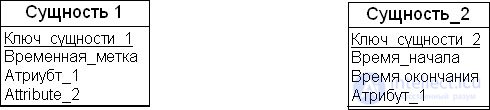
There are two main types of timestamps — point-in-time timestamps, or instant timestamps (Instant timestamp), and range timestamps, or interval timestamps (Interval timestamp).

An instant timestamp is a single-valued timestamp that represents a moment in time. Such timestamps are used to represent, in a data warehouse, objects that change over time, such as business operations or events. They are also used to record changes to data values extracted from operational systems and then stored in the data warehouse.

Interval timestamps represent a period or range of time and usually contain two values: the start and end of the period, or the length of the interval. Such timestamps are typically used to model the state of an object and its behavior over time. If the length of the interval is fixed — for example, a day or a month — a single value can be used to represent the interval timestamp.

Fig. 7.2 shows examples of entities defined with an instant timestamp (Entity_1) and with interval timestamps (Entity_2).

Fig. 7.2. Defining entities with instant and interval timestamps

The need to account for the time element in a data model presents the data warehouse designer with the following tasks.

1. Choosing an approach to modeling temporal data.
2. Defining the domain of the "time" attribute.
3. Defining the structure of the "time" attribute's domain.
4. Defining the timestamp attributes.
5. Normalizing time dependencies.
6. Choosing what to model — states or events?
7. Mapping the temporal data model onto the original static data model.

To model temporal data for a domain, the model must be extended by introducing temporal (time-related) entities or relationships. Such an extension can be made in various ways.

Currently, the following approaches are the most widely used for building a temporal data model:

• accumulating snapshots, or cumulative snapshots (Cumulative snapshots);
• maintaining a history of data changes, or a continuous history model (Continuous history model) – event and state tables.

Let us now look at each of these approaches in more detail.

The Snapshot-Table Model

The approach to modeling temporal data based on accumulating snapshots consists of collecting snapshots of a fragment of the domain and accumulating such snapshots in various fragments of the database, or in another database, as a life history of the domain's data. For example, if snapshots are captured at the end of each day, the set of snapshots collected over a period will represent the day-by-day change in the picture of the domain data maintained in the database.

A relational database table that represents snapshots is called a snapshot table (Snapshot Table). Let us look at an example of such a table (Table 7.1). It contains no timestamps. A designer may add a timestamp using user-defined time. This table represents instances of domain entities as they exist at a given moment in time. Updating a relational database table is a destructive operation – no history of data changes over time is maintained.

Table 7.6 shows the contents of the snapshot table (Empl) before and after an update.

Polyanova E.S.

Below are examples of SQL data manipulation statements against the Empl snapshot table.

Deleting a table row:

DELETE FROM Empl WHERE Name = 'Полянова Е.С.';

Adding a row to the table:

INSERT INTO Empl VALUES ('Маски А.С.','МАС','12000');

Updating a table row:

UPDATE Empl SET Dept = 'МАС', Sal ='11500' WHERE Name = 'Полянова Е.С.';

The cumulative-snapshot method is also used outside the context of temporal data modeling. It is simple and easy to understand, but it has a number of drawbacks. The first drawback is data redundancy, which arises from periodically reloading data from the data source. As a result, the size of the data warehouse grows quickly. To mitigate this, data aggregation with summed metrics, or snapshot versioning, is often used.

The second drawback of this approach is the possible loss of information. This drawback stems from the problem of synchronizing changes in the state of data at the data sources with the moment the snapshot is captured in the warehouse. Reflecting changes in the state of domain data in the warehouse is one of the hardest problems a data warehouse designer must solve. Within a snapshot-based approach, this problem can be quite difficult to solve. For example, if data needs to be captured every second, the volume of data in the warehouse will grow so quickly that the warehouse project becomes prohibitively expensive. Such situations can arise in domains related to auditing exchange-trading operations.

The Event-Table Model

Building a continuous history model aims to create a data model that reflects the history of data changes in the warehouse. This model is more complex than the cumulative-snapshot model, including in terms of interpreting it. Nevertheless, the continuous history model is more relevant for analyzing time series of domain parameters.

The approach to modeling temporal data based on recording domain events consists of adding a timestamp that captures the event (fact) as an attribute of the domain entity instance, and reflecting the moment in time in a database table as the life history of the domain's data. For example, tracking a customer's bill payments.

A relational database table that represents domain events is called an event table (Event Table). Let us look at an example of such a table for tracking a customer's bill payments (Table 7.7). An event for the "Invoice" domain entity consists of creating an entity instance containing data indicating that the customer paid an invoice for a certain amount at a certain time. The timestamp in this table records the time the customer paid the invoice, i.e., it represents the valid time of the payment fact. A designer may add a user-defined-time timestamp to such a table. Among other things, the data in this table supports the history of bill payments by a specific customer. This table's data is never updated, since it is intended only to accumulate data (insert operations only).

Event tables are typically used to represent data that must be summarized, i.e., aggregated over various periods of time.

The State-Table Model

The approach to modeling temporal data based on recording domain states consists of adding timestamps that mark the start and end of a particular state as attributes of the domain entity instance, and reflecting the start and end moments of a particular entity state in a database table as the life history of the domain's data.

A relational database table that represents the state of domain objects is called a state table (State Table). A state refers to objects that exist during a specific period of time. An example of a state table (Empl) is given in Table 7.8. The table's rows are data on employee salaries in an organization, together with the period of time during which the given salary was paid, i.e., the state of the "Employee" entity instance is preserved. The pair of timestamps "Assignment time" and "Cancellation time" defines the period of time during which the table row is meaningful. The value FOREVER equals the largest time value accepted by the system.

Below are the SQL data manipulation statements for the Empl state table.

Adding a row to the table:

INSERT INTO Empl VALUES ('Рыков А.С.','МИК','12000',
'02.02.2009', FOREVER);

Updating a table row (note that the update consists of two actions:

1. setting the cancellation time to the time specified in the organization's order, and
2. adding a new row with an assignment time equal to the time specified in the organization's order, and a cancellation time equal to FOREVER ).

UPDATE Empl SET EDate="30.05.2008" WHERE Name = 'Амосова Е.С.'
AND Edate=FOREVER;
INSERT INTO Empl VALUES ('Амосова Е.С.','МИК','12000',
'01.06.20089', FOREVER);

As a rule, rows are deleted from state tables only after data processing has been completed and after the archiving process.

Like event tables, state tables are used to store data that must be summarized, i.e., aggregated over various periods of time. Note that in an event table, summation is performed over a single period of time, whereas in a state table the given period may overlap with the periods of particular entities, and consequently, when aggregating data, it may be necessary to split the given period into several sub-periods to account for the existing overlap between row periods.

Formulating Queries Against Temporal Data

Designing queries that use timestamps requires particular care and precision from the designer. Let us look at how typical predicates are formulated using timestamps, namely predicates comparing periods of time. Let Р1 be the time interval "P1Start, Р1End", and P2 — the time interval "P2Start, Р2End". Let us also introduce the notation VALID(T) to denote the period of time in a table row. Note that a period of time is not a scalar quantity — and this is precisely what creates certain difficulties in formulating predicates for comparing periods of time. If instant timestamps are being compared, the standard set of SQL scalar comparison operators is used for the DATA or TIMESTAMP data type.

If P1Start < P2Start, we have the "Less than" predicate for comparing periods of time: P1 < P2 (Fig. 7.3). If P1End > P2End, we have the "Greater than" predicate for comparing periods of time: P1 > P2. If P1Start = P2Start AND P1End = P2End, the periods of time are considered equivalent. This type of predicate is used to order periods of time.

Fig. 7.3. The "Less than" predicate for comparing periods of time

Let us consider the "Precedes" predicate for comparing periods of time (denoted in examples as PRECEDES), which holds when one period of time precedes another (Fig. 7.4): the condition P1End < P2Start holds. This type of predicate is used to separate periods of time.

Fig. 7.4. The "Precedes" predicate for comparing periods of time

To find the periods of time during which the value of a fact changes, the time-period comparison predicate "Meets" is used (notation used in the examples — MEETS ). If time period P2, roughly speaking, latches its start onto the end of period P1, then the logical condition (P1End = P2Start – 1) OR (P2End = P1Start – 1) holds (see fig. 7.5). An example of using such a predicate would be queries like "the price of a product is rising or falling," "salary was increased," and so on.

enlarge image
Fig. 7.5. Time-period comparison predicate "Meets"

An SQL statement to select the list of price changes for a product from table Table1 might look like this:

SELECT B.No, B.Price. A.Price
FROM Table1 A, Table1 B
WHERE A.No=B.No AND A.Price < B.Price
AND VALID(A) PRECEDES VALID(B) AND VALID(A) MEETS VALID(B)

Combining temporal predicates means that we first order the time periods, and then chain them one after another. This produces a continuous timeline of periods.

To find intersections of time periods, the time-period comparison predicate "Overlaps" is used (notation used in the examples — OVERLAPS ). If time period P1 intersects time period P2, then the logical condition (P1Start <= P2End) OR (P2Start <= P1End) holds. An example of using such a predicate is a query like "Find all employees who worked at the organization during the period from January 1, 2008 to February 20, 2009," for example (table 7.7):

SELECT Name FROM Empl WHERE VALID(Empl) OVERLAPS [01.01.2008,
20.02.2009]

To find events that occurred during a specific period of time, the time-period comparison predicate "Contains" is used (notation used in the examples — CONTAINS ). If time period P1 is contained within time period P2, then the logical condition (P1Start <= P2Start) OR (P1End <= P2End) holds (see fig. 7.6).

Fig. 7.6. Time-period comparison predicate "Contains"

There are several types of queries against temporal data for state tables.

• Snapshot queries (Snapshot query) – queries that build a selection of table rows valid at a specific point in time (date).
• Nonsequenced temporal queries (Nonsequenced temporal query) – queries that build a selection of table rows without regard to timestamps, i.e., the resulting rows have no time-based relationship to one another. The result is a snapshot table.
• Sequenced temporal queries (Sequenced temporal query) — queries that build a selection of table rows for a specific period of time using the time-period comparison predicates discussed above. The result is a state table in which the timestamp for each tuple satisfies certain temporal constraints.

Let's give an example of a sequenced temporal query. Consider the database tables Employee (Empl) and Department (Department), the contents of which are given in tables 7.9 and 6.10. Let's build a query to answer the question "Who managed the department of Prokhorov A.I.?" The result is given in table 7.11.

SELECT Manager FROM Empl, Department
WHERE Department.Dept = Empl.Dept AND Empl.Name ='Прохоров А.И.'
AND VALID(Empl) OVERLAPS VALID(Department)

Now let's look at the main techniques for modeling temporal data.

Main techniques for modeling temporal data

Accounting for the domain's time dependencies

Let's look at techniques for applying temporal data modeling in practice. Consider an example database about video films ("Film"), recorded at particular studios ("Studio") under the direction of particular managers ("Director") with the participation of particular actors ("Actor"). A fragment of the logical structure (ER model) linking the entities above is shown in fig. 7.7. This ER model is static — it does not account for any historical aspects of a studio's existence or the time a particular manager spent working on a particular picture.

enlarge image
Fig. 7.7. ER model of a video-film database without accounting for time dependencies

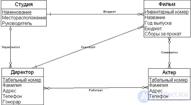
Suppose the data warehouse designer is tasked with building a historical model for the given ER model using temporal data modeling methods. The designer must examine the time dependencies of the domain's entities and incorporate them into the static ER model. A time dependency is a functional dependency of the values of a domain entity's attributes on time.

To account for time dependencies, the designer needs to add timestamps to the static structure given above. In doing so, the designer must address the following tasks:

• based on the task at hand, decide which entities' behavior over time will be accounted for in the model, and which will not;
• determine whether there are entities that may contain timestamps that are semantically meaningful for the domain, and interpret them accordingly;
• add timestamps to the entities of the ER model. In doing so, a decision must be made about how the entity will be modeled – using events or states. Events are used to account for operations that change data at certain points in time. States are used to represent the state of an entity's attributes over a given period of time. In the first case, instant (point-in-time) timestamps are used, and in the second, interval timestamps are used;
• define the domains of the timestamps based on the "date/time" type available in the DBMS, and strictly adhere to these domain definitions going forward.

When addressing these tasks, relationships between entities are temporarily left out of consideration.

Suppose that in our example the customer is not interested in the history of the relationships between actors and the managers (directors) of films, nor in the history of actors' participation in various films. Then temporal data modeling will not be performed for the entity describing actors.

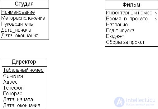
Further, suppose the customer is interested in the history of a studio's state or in the periods during which film managers were employed. Then it is natural to model the temporal behavior of the entities describing studios and managers by recording the state of their attributes.

Suppose the customer is interested in the history of a film's theatrical run. Then it would make sense to perform temporal modeling of the entity describing the film by recording the events associated with the film.

For example, one of the business applications the customer needs will be "Video Rental." Customers pay to use a videotape for a certain amount of time and number of days. The application keeps track of providing such services to customers.

The result of temporal modeling on the ER model is shown in fig. 7.8 below.

Fig. 7.8. Adding timestamps to the entities of the static ER model

Thus, the main technique of logical modeling of a domain's temporal data is adding timestamps to the domain's entities. Adding timestamps to the entities of the logical model makes it possible to record, in the model, the behavior of certain entity attributes over time. Such entity attributes form time dependencies of attributes.

Classes of attribute time dependencies (model normalization)

After adding timestamps to the entities of the logical model, one of the designer's main tasks becomes identifying the entity attributes that participate in the time dependency. One technique for solving this problem within the relational data model is normalization of time dependencies, or building classes of time dependencies (Volatility Classes).

A time dependency class is a group of entity attributes that jointly change their values over time. The answer to the question of how many attributes should fall into a class is not clear-cut. Classes with a small cardinality of attributes are impractical, while grouping a large number of independently time-varying attributes into a single class increases storage redundancy. A good practical criterion is the complexity of maintaining these classes in the data warehouse.

In practice, temporal data model designers use the following two main classes:

• the class of time-independent attributes (Time-invariant Volatility Class);
• the class of time-dependent attributes (Time-variant Volatility Class).

The class of time-independent attributes consists of either attributes that do not depend on time, or attributes for which a decision has been made not to store the history of their temporal behavior. This class is always non-empty, since it is assumed that the entity's key is made up of attributes that do not depend on the entity's temporal relationships within the domain.

The attributes of this class are placed in a new entity, which represents a part of the original entity. This new entity essentially becomes the root of a hierarchy of temporal relationships with all the time-dependent entities derived from the original entity. From this perspective, the history of the entity's behavior over time can be modeled through its dependent entities.

For example, for the entity "Film Director," the attributes Employee ID, Last Name, Address, and Phone are candidates for inclusion in the class of time-independent attributes. Clearly, this assumes the director will not change their last name, and we are not interested in the history of their place of residence.

For the entity "Film," such a class might consist of the attributes Inventory number of the film, Title of the film, and Release year of the film.

The class of time-dependent attributes consists of those entity attributes that change synchronously over time. An entity may have several such classes. Each such class must be moved out into a separate entity.

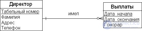
For example, for the entity "Film Director," the class of time-dependent attributes will consist of the interval timestamp and the director's Salary. This will be the only such class for the original entity. Here, as the designer has already decided, the history of the state of the Salary attribute will be modeled. Fig. 7.9 below shows the historical model for the entity "Film Director."

Fig. 7.9. Temporal logical model for the entity "Film Director"

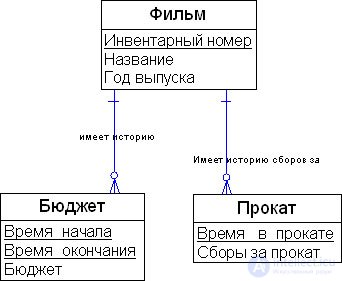
For the entity "Film," two classes of time-dependent attributes can be identified, since the values of the attributes Budget of the film and Rental revenue behave independently of one another over time. Moreover, since the value of the Budget attribute does not change very often, it is reasonable to use a state model with an interval timestamp for modeling its behavior over time. The value of the Rental revenue attribute changes with every data write to the data warehouse, and consequently this event must be reflected using an instant timestamp. The resulting logical model of the historical behavior of the "Film" entity is shown in fig. 7.10 below.

Fig. 7.10. Temporal logical model for the entity "Film"

Having examined the original logical model with respect to accounting for the behavior of entities over time, the data warehouse designer must answer the question of whether all the temporal data that needs to be stored in the data warehouse has been accounted for (if not, then the corresponding entities of the logical model must be built).

Solving this problem is usually associated with searching for entities to represent business events and operations that are important for data-analysis tasks in the data warehouse but are not supported within the original ER model of the source OLTP systems. This task is quite complex and requires a thorough study of the domain from the perspective of data analysis.

Thus, in our example we did not consider a number of questions related to actors' participation in films. End users may be interested in a number of questions related to the "Actor" entity:

• Which actors does a given director work with most often?
• Which actors does a given director not use more than once?
• How do actors' fees change as their popularity grows?
• Which roles is a given actor invited to play most often?

If a user can get answers to the first two questions using the existing ER model's data structure (see fig. 7.7), then to answer the other two, the logical model must be supplemented with information about actors' fees in films and a metric measuring an actor's popularity. Whether additional attributes or entities are needed to represent such information is a decision for the data warehouse designer.

Thus, normalization of the temporal logical model is based on identifying classes of time-dependent attributes and moving them out into separate domain entities.

Now we are ready to proceed to building the logical temporal model of the video-film data warehouse domain.

Building the logical temporal data model

After the designer has built temporal models for the entities of the original ER model, the next step is to gather all the entities' temporal models into a single logical data model and record all the necessary relationships.

For each relationship in the original logical model, the data warehouse designer must investigate the question: does the history of the relationship need to be stored in the data warehouse? If the history of changes to the relationship does not need to be preserved in the data warehouse, then the relationship is simply carried over into the constructed temporal model of entities as a relationship between the entities representing the classes of time-independent attributes.

If the history of changes to the relationship needs to be preserved in the data warehouse, then that relationship needs to be supplemented with timestamp attributes, representing it as an entity. In the relational data model, a relationship between entities is modeled by means of relations and, consequently, must be represented using entities.

For the example we are considering, the temporal data model might look like the one in fig. 7.11. As can be seen from the figure, the four original relationships (owns, employs, works, and has) have been carried over into the temporal data model from the ER model unchanged, since it was decided not to preserve information about their temporal behavior.

enlarge image
Fig. 7.11. Temporal data model of the video-film database

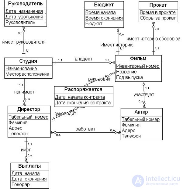
For the "Studio" entity, it was decided to store the history of changes of its directors, so the "Studio Director" entity was added to the model. Temporal models for the "Film" and "Director" entities were built earlier, and their relationships with other entities in the model have been recorded. But the "manages" relationship from the original ER model is represented as the "Manages" entity (a film), since it was decided to preserve the history of managers' work on films.

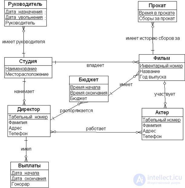
The data warehouse designer can further examine the resulting model in order to reduce its complexity, for example by reducing the number of entities in the model. In our case, it is easy to notice that the period during which a manager works on a film coincides with the period during which the film has been allocated funding. Consequently, the "Manages" and "Budget" entities can be merged into a single "Budget" entity, as shown in fig. 7.12. This technique is called grouping of time-dependent attribute classes. Note that using this technique increases data redundancy in the model.

enlarge image
Fig. 7.12. Transformation of the resulting temporal data model of the video-film database

Thus, certain temporal constraints, those that contain a temporal aspect, are represented in the model as relationship entities. However, there are temporal constraints that are expressed as business rules. Such constraints are hard to model within an extended ER model that maps to the relational model using standard design rules. For example, there might be a business rule: two managers cannot work on the same film at the same time. Such business rules are usually formulated using descriptive text and are used by application developers, i.e., they are modeled in the database application's code.

It should also be noted that temporal constraints should be recorded in the metadata dictionary, since they are important information for the end user.

Thus, the logical temporal model of the video-film data warehouse domain has been built.

Summary

The approach to modeling temporal data discussed in this lecture is an extension of the entity-relationship model that accounts for the time dependencies of certain attributes of domain entities.

With this approach, the designer performs the following sequence of actions.

• Develops an entity-relationship model for the selected domain (ER diagrams, typically in third normal form) without accounting for the time dependencies of the model's attributes.
• Based on business requirements, determines which model attributes are time-dependent and will be accounted for in the model being developed (i.e., decides on the set of temporal data to include in the model).
• Accounts for attribute time dependencies by introducing timestamps into the entities.
• Normalizes the resulting temporal entities by identifying classes of time-dependent attributes and moving them out into separate entities.
• Decides how to represent the domain's relationships (including time-dependent ones) as domain entities.
• Gathers the resulting entities into a single ER model. This model is, as a rule, normalized.
• Decides on denormalizing the model, based on query performance requirements or on well-founded considerations for simplifying the model (for example, clarity).

As a result of applying temporal modeling, the designer creates a logical model of the domain that accounts for the time dependencies of the data, independent of the specific hardware/software implementation. This method is used both when modeling the domains of OLTP systems and when modeling the domains of BI systems.

Knowledge of the techniques for building logical temporal data models is especially important when designing a data warehouse, since one of the goals of building one is to study the time dependencies of the organization's data.

See also

• Relational data warehouses
• [[b4470]]
• [[b6923]]
• [[b9333]]
• [[b9334]]
• [[b9335]]
• The "Data Vault" modeling method
• [[b5835]]
• [[b148]]
• [[b9335]]
• [[b152]]
• [[b5828]]
• [[b148]]

See also

• 8. Elements of the model "entity-relationship" ER-diagrams in databases
• The concept of data storage (DS). Differences between data warehouses and databases
• The entity-relationship modeling method
• The dimensional modeling method
• Temporal data modeling methods
• 4. Models
• Modeling. Introduction
• Temporal data modeling methods
• Psychological modeling
• Simulation
• Modeling. Introduction