Window functions in SQL

Many developers, even those who've known SQL for years, don't understand window functions, treating them as some kind of special magic reserved for the chosen few. And even though window function support has been available since SQL Server 2005, some people still «copy-paste» them from StackOverflow without going into the details. In this article we'll try to dispel the myth that this SQL feature is somehow inaccessible, and show a few examples of window functions in action on a real dataset.

In a regular query, the whole set of rows is processed as a single «solid block», for which aggregates are computed. With window functions, the query is instead split into parts (windows), and aggregates are computed separately for each of these parts.

Why not GROUP BY or JOIN

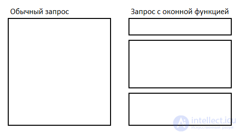
Let's clarify right away that window functions are not the same thing as GROUP BY. They don't reduce the number of rows — they return as many values as they received on input. Second, unlike GROUP BY, OVER can reference other rows. And third, they can compute moving averages and cumulative sums.

Note: Window functions don't change the result set — they only add some extra information to it. To make this easier to understand, you can think of SQL as first executing the whole query (except for sorting and limit), and only afterward computing the window values.

Okay, we've sorted out GROUP BY. But in SQL there are almost always several ways to reach the same goal. For instance, you might be tempted to use subqueries or JOIN. Of course, JOIN is preferable to subqueries in terms of performance, and the performance of JOIN and OVER constructs turns out to be the same. But OVER gives you more freedom than a rigid JOIN. And the amount of code ends up being much smaller.

Getting started

A window function is a SQL function in which the input values are taken from a "window" of one or more rows in the result set of a SELECT statement.

Window functions differ from other SQL functions in that they have an OVER clause. If a function has an OVER condition, it's a window function. If it lacks an OVER condition, it's an ordinary aggregate or scalar function. Window functions may also have a FILTER clause between the function and the OVER clause.

Window functions start with the OVER operator and are configured using three other operators: PARTITION BY, ORDER BY and ROWS. We'll go into more detail about ORDER BY, PARTITION BY, and its helper operators LAG, LEAD, and RANK.

The syntax looks roughly like this:

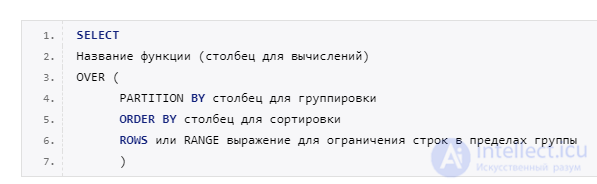
A window is an expression describing the set of rows that the function will process and the order of that processing.
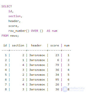
Note that a window can simply be specified with empty parentheses (), meaning the window is all rows of the query result.

For example, in this SELECT, row numbering is simply added on top of the regular id, header, and score fields.

You can add ORDER BY inside the window expression, which lets you change the order of processing.

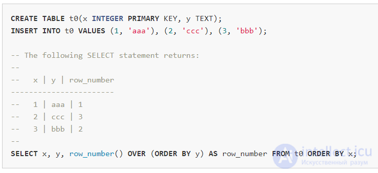
The row_number() window function assigns each row a sequential integer in the order specified by the "ORDER BY" clause inside the window-defn (in this case "ORDER BY y"). Note that this does not affect the order in which results are returned from the overall query. The order of the final result is still governed by the "ORDER BY" clause attached to the SELECT statement (in this case "ORDER BY x").

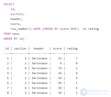
Note that I also added ORDER BY id at the end of the whole query, and the ranking is still computed correctly. In other words, the DBMS simply sorted the result together with the output of the window function — one order clause doesn't interfere with the other in any way.

Unlike ordinary functions, window functions cannot use the DISTINCT keyword. Furthermore, window functions can only appear in the result set and in the ORDER BY clause of a SELECT statement.

There are two kinds of window functions: aggregate window functions and built-in window functions. Every aggregate window function can also work as an ordinary aggregate function simply by omitting the OVER and FILTER clauses. Moreover, all of SQLite's built-in aggregate functions can be used as an aggregate window function by adding the appropriate OVER clause. Applications can register new aggregate window functions using the sqlite3_create_window_function() interface. However, built-in window functions require special handling in the query planner, and consequently new window functions exhibiting the exceptional properties found in built-in window functions cannot be added by an application.

An aggregate window function is similar to an ordinary aggregate function, except that adding it to a query doesn't change the number of rows returned. Instead, for each row, the result of the aggregate window function is as if the corresponding aggregate were computed over all the rows in the «window frame» specified in the OVER clause.

It goes further still. You can add the word PARTITION BY [expression] to the window expression,
for example row_number() OVER (PARTITION BY section), and then the count will be computed separately within each group:

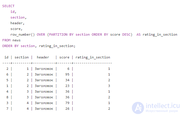
If no partition is specified, the partition is the entire query result.

Here we need to say a bit right away about which functions can be used, since there's a very important nuance.
As a function you can use, so to speak, the "true" window functions from the manual — these are

row_number(),

rank(),

lead(), and so on, or you can use aggregate functions such as: sum(), count(), and so on.

Now, this is important — aggregate functions work a little differently: if no ORDER BY is specified within the window, the calculation runs over the whole partition once, and the result is written into every row (the same for all rows of the partition). But if ORDER BY is specified, the calculation for each row runs from the start of the partition up to that row.

All the examples will be based on Datacamp's Olympic medalists dataset. The table is called summer_medals and contains the results of the Olympics from 1896 to 2010:

ROW_NUMBER and ORDER BY

As mentioned above, the OVER operator creates a window function. Let's start with the simple ROW_NUMBER function, which assigns a number to each selected record:

SELECT
athlete,
event,
ROW_NUMBER() OVER() AS Row_Number
FROM Summer_Medals
ORDER BY Row_Number ASC;

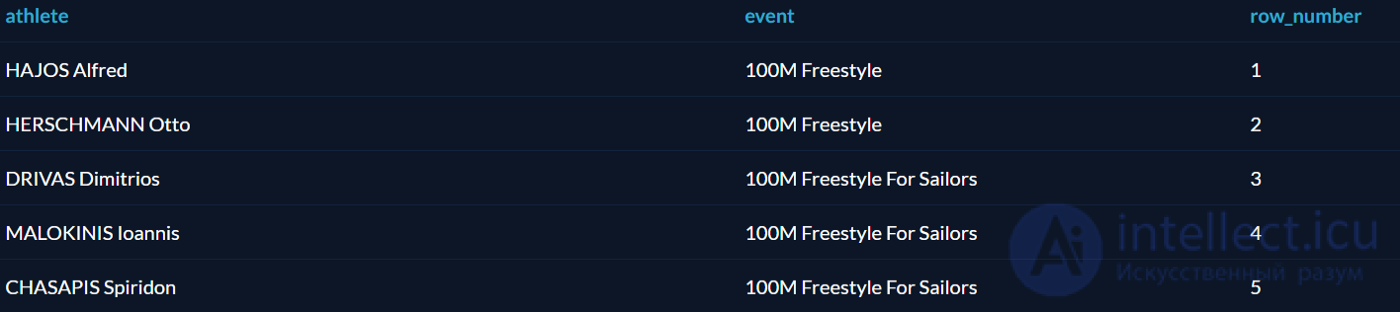
Each «athlete — event» pair got a number, and these numbers can be referenced by the name row_number.
ROW_NUMBER can be combined with ORDER BY to determine the order in which rows are numbered. Let's use DISTINCT to select all the available sports and number them in alphabetical order:

SELECT
sport,
ROW_NUMBER() OVER(ORDER BY sport ASC) AS Row_N
FROM (
SELECT DISTINCT sport
FROM Summer_Medals
) AS sports
ORDER BY sport ASC;

PARTITION BY and LAG, LEAD, and RANK

PARTITION BY lets you group rows by the value of a particular column. This is useful when the data logically splits into some categories and you need to do something with a given row relative to the other rows in the same group (say, compare a tennis player to other tennis players, but not to runners or swimmers). This operator only works with window functions like LAG, LEAD, RANK, and so on.

LAG

The LAG function takes a row and returns the one that preceded it. For example, suppose we want to find all Olympic tennis champions (men and women separately) starting from 2004, and for each of them determine who the previous champion was.
Solving this requires a few steps. First, we need to create a common table expression that stores the result of the "tennis champions since 2004" query as a temporary named structure for further analysis. Then we split them by gender and select the previous champion using LAG:

– Табличное выражение ищет теннисных чемпионов и выбирает нужные столбцы
WITH Tennis_Gold AS (
SELECT
Athlete,
Gender,
Year,
Country
FROM
Summer_Medals
WHERE
Year >= 2004 AND
Sport = 'Tennis' AND
event = 'Singles' AND
Medal = 'Gold')

– Оконная функция разделяет по полу и берёт чемпиона из предыдущей строки
SELECT
Athlete as Champion,
Gender,
Year,
LAG(Athlete) OVER (PARTITION BY gender
ORDER BY Year ASC) AS Last_Champion
FROM Tennis_Gold
ORDER BY Gender ASC, Year ASC;

The PARTITION BY clause returned all the men first, then all the women. For the 2008 and 2012 winners the previous champion is shown; since we only have data for 3 Olympics, the 2004 champions have no predecessor, so those fields contain null.

LEAD

The LEAD function is similar to LAG, but instead of the previous row it returns the next one. We can find out who became the next champion after a given athlete:

– Табличное выражение ищет теннисных чемпионов и выбирает нужные столбцы
WITH Tennis_Gold AS (
SELECT
Athlete,
Gender,
Year,
Country
FROM
Summer_Medals
WHERE
Year >= 2004 AND
Sport = 'Tennis' AND
event = 'Singles' AND
Medal = 'Gold')

– Оконная функция разделяет по полу и берёт чемпиона из следующей строки
SELECT
Athlete as Champion,
Gender,
Year,
LEAD(Athlete) OVER (PARTITION BY gender
ORDER BY Year ASC) AS Future_Champion
FROM Tennis_Gold
ORDER BY Gender ASC, Year ASC;

RANK

The RANK operator is similar to ROW_NUMBER, but it assigns the same numbers to rows with the same values, and skips the "extra" numbers. There's also DENSE_RANK, which doesn't skip numbers. That sounds confusing, so it's easier to show with an example. Here's a ranking of countries by the number of Olympics they participated in, using different operators:

• Row_number — nothing interesting here, the rows are simply numbered in ascending order.
• Rank_number — the rows are ranked in ascending order, but there's no number 3. Instead, 2 rows share number 2, followed immediately by number 4.
• Dense_rank — the same as rank_number, but number 3 isn't skipped. The numbers run consecutively, but then no one ends up being fifth out of five.

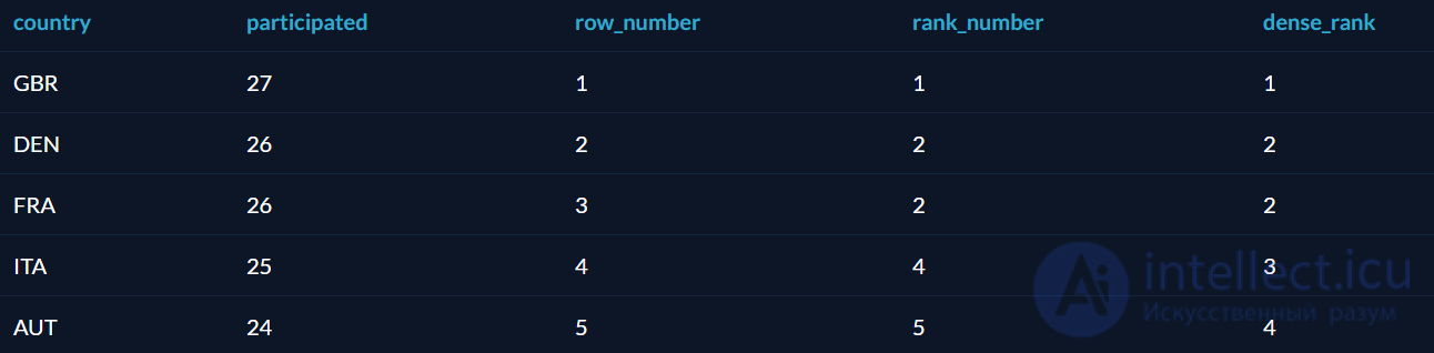
Here's the code:

-- Табличное выражение выбирает страны и считает годы
WITH countries AS (
SELECT
Country,
COUNT(DISTINCT year) AS participated
FROM
Summer_Medals
WHERE
Country in ('GBR', 'DEN', 'FRA', 'ITA','AUT')
GROUP BY
Country)

-- Разные оконные функции ранжируют страны
SELECT
Country,
participated,
ROW_NUMBER()
OVER(ORDER BY participated DESC) AS Row_Number,
RANK()
OVER(ORDER BY participated DESC) AS Rank_Number,
DENSE_RANK()
OVER(ORDER BY participated DESC) AS Dense_Rank
FROM countries
ORDER BY participated DESC;

Frame type

There are three frame types: ROWS, GROUPS, and RANGE. The frame type determines how the starting and ending frame boundaries are measured.

• ROWS: the ROWS frame type means that the starting and ending frame boundaries are determined by counting individual rows relative to the current row.

• GROUPS: the GROUPS frame type means that the starting and ending boundaries are determined by counting «groups» relative to the current group. A «group» is a set of rows that all have equivalent values for every term of the window's ORDER BY clause. («Equivalent» means the IS operator is true when comparing the two values.) In other words, a group consists of all peers of a row.

• RANGE: the RANGE frame type requires that the window's ORDER BY clause have exactly one term. Call this term «X». With the RANGE frame type, frame elements are determined by computing the value of expression X for every row in the partition and framing those rows for which the value of X falls within a certain range of the value of X for the current row. See the description of the «PRECEDING» boundary specification below for more details.

The ROWS and GROUPS frame types are similar in that they both determine the extent of the frame by counting relative to the current row. The difference is that ROWS counts individual rows, while GROUPS counts peer groups. The RANGE frame type is different: it determines the extent of the frame by finding expression values that fall within a certain range of values relative to the current row.

Syntax

A window is defined using the mandatory OVER() clause. Let's look at the syntax of this clause:

Now let's break down how a set of rows behaves when using one keyword or another. We'll practice on a simple table containing a date, the channel the user came from, and the number of conversions:

OVER()

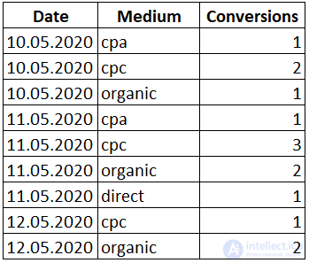
Let's open a window using OVER() and sum the «Conversions» column:

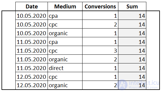
We used the OVER() clause with no arguments. In this case the window is the entire dataset and no sorting is applied. A new column «Sum» appeared, and the same value, 14, is output for every row. This is the running total of all the values in the «Conversions» column.

PARTITION BY

Now let's apply the PARTITION BY clause, which specifies the column by which grouping is performed and is the key to splitting the set of rows into windows:

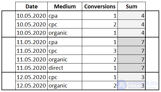
The PARTITION BY clause grouped the rows by the «Date» field. Now a separate sum of the «Conversions» column is calculated for each group.

ORDER BY

Let's try sorting the values within the window using ORDER BY:

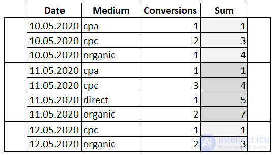
We added ORDER BY on the «Medium» field to the PARTITION BY clause. This way we specified that we want to see, not the sum of all values in the window, but for each «Conversions» value, the sum together with all the preceding ones. In other words, we computed a running total.

ROWS or RANGE

The ROWS clause lets you restrict the rows in the window by specifying a fixed number of rows preceding or following the current one.

The RANGE clause, unlike ROWS, doesn't work with rows but with a range of rows in the ORDER BY clause. That is, for RANGE, several physical rows with the same rank can be treated as a single row.

Both ROWS and RANGE clauses are always used together with ORDER BY.

In the expression restricting rows for ROWS or RANGE, you can also use the following keywords:

• UNBOUNDED PRECEDING — specifies that the window starts at the first row of the group;
• UNBOUNDED FOLLOWING – this clause specifies that the window ends at the last row of the group;
• CURRENT ROW – specifies that the window starts or ends at the current row;
• BETWEEN «window boundary» AND «window boundary» — specifies the lower and upper bound of the window;
• «Value» PRECEDING – specifies the number of rows before the current row (not allowed in the RANGE clause);
• «Value» FOLLOWING — specifies the number of rows after the current row (not allowed in the RANGE clause).

Let's look at an example:

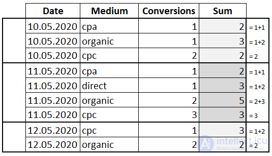
In this case, the sum is computed over the current cell and the next one in the window. And the last row in the window has the same value as the «Conversions» column, because there's nothing left to add.

By combining these keywords, you can tailor the range a window function operates over to your specific task.

Types of window functions

Window functions can be divided into the following groups:

• Aggregate window functions;
• Ranking window functions;
• Offset window functions;
• Analytic window functions.
• User-defined window functions

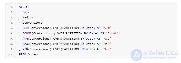
You can use several window functions at once in a single SELECT statement with a single FROM clause. Let's go through each group in detail and cover the main functions.

Aggregate functions

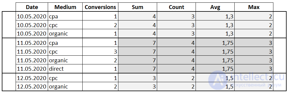
Aggregate functions are functions that perform arithmetic computations over a dataset and return a final value.

• SUM – returns the sum of the values in a column;
• COUNT — counts the number of values in a column (NULL values are not counted);
• AVG — determines the average value in a column;
• MAX — determines the maximum value in a column;
• MIN — determines the minimum value in a column.

An example of using aggregate functions with the OVER window clause:

Ranking functions

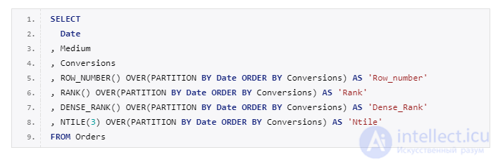
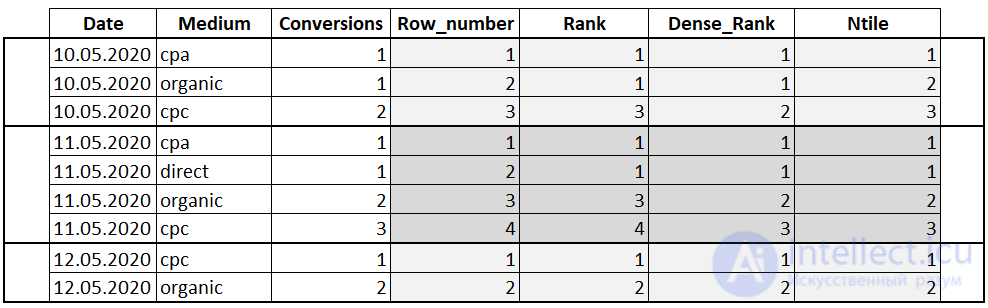
Ranking functions are functions that rank the value for each row in a window. For example, they can be used to assign a sequence number to a row or to build a rating.

• ROW_NUMBER – the function returns the row number and is used for numbering;
• RANK — the function returns the rank of each row. Here the values are already analyzed, and if identical ones are found, it returns the same rank while skipping the next value;
• DENSE_RANK — the function returns the rank of each row. But unlike RANK, for identical values it returns a rank without skipping the next one;
• NTILE – a function that lets you determine which group the current row belongs to. The number of groups is specified in parentheses.

Offset functions

Offset functions are functions that let you move to and access different rows in a window relative to the current row, as well as access values at the beginning or end of the window.

• LAG or LEAD – the LAG function accesses data from the previous row in the window, and LEAD accesses data from the next row. The function can be used to compare the current row's value with the previous or next one. It takes three parameters: the column whose value should be returned, the number of rows to offset by (default 1), and the value to return if the offset would return NULL;
• FIRST_VALUE or LAST_VALUE — these functions let you get the first and last value in the window. They take as a parameter the column whose value should be returned.

Analytic functions

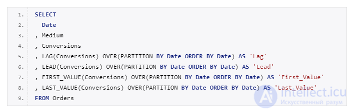
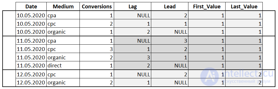
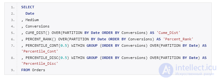
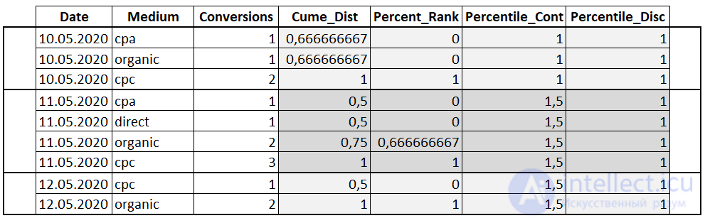
Analytic functions are functions that return information about the distribution of data and are used for statistical analysis.

• CUME_DIST — computes the cumulative distribution (relative position) of values in the window;
• PERCENT_RANK — computes the relative rank of a row in the window;
• PERCENTILE_CONT — computes a percentile based on a continuous distribution of the column's value. It takes as a parameter the percentile to compute (in this article I show how to calculate the median using this function);
• PERCENTILE_DISC — computes a specific percentile for sorted values in a dataset. It takes as a parameter the percentile to compute.

Important! For the PERCENTILE_CONT and PERCENTILE_DISC functions, the column to sort by is specified using the WITHIN GROUP keyword.

Case study. Attribution models

An attribution model lets you make a reasoned assessment of each channel's contribution to reaching a conversion. Let's try computing two different attribution models using window functions.

We have a table with a visitor id (this could be a Client ID, phone number, etc.), dates and the number of site visits, as well as information about conversions achieved.

First click

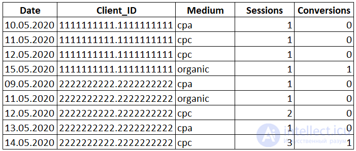
In Google Analytics, the default attribution model is last non-direct click. In this case, 100% of the conversion's value is assigned to the last channel in the interaction chain.

Let's try computing the first-interaction model, where 100% of the conversion's value is assigned to the first channel in the chain, using the FIRST_VALUE function.

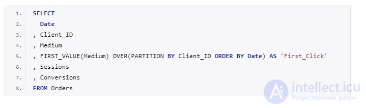
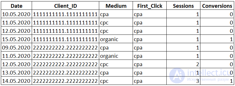
Next to the «Medium» column, a new column «First_Click» appeared, showing the channel that first brought the visitor to our site, and the full value is credited to that channel.

Let's aggregate the data and get a report.

Accounting for interaction recency

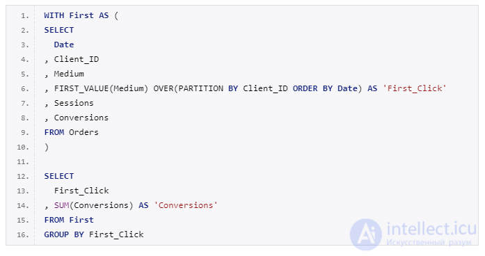
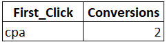
Here the rule that applies is: the closer an interaction point is to the conversion, the more valuable it's considered to be. Let's try to compute this model using the DENSE_RANK function.

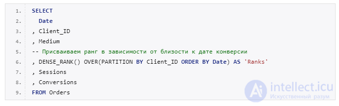
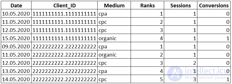
Next to the «Medium» column, a new column «Ranks» appeared, showing the rank of each row based on its proximity to the conversion date.

Now let's use this query to distribute a value of 1 (100%) across all the touchpoints on the path to conversion.

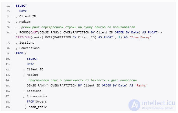
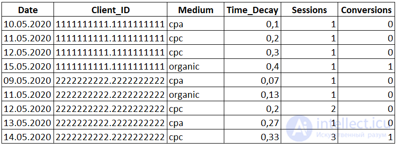
Next to the «Medium» column, a new column «Time_Decay» appeared with the distributed value.

And now, if we aggregate, we can see how the value was distributed across channels.

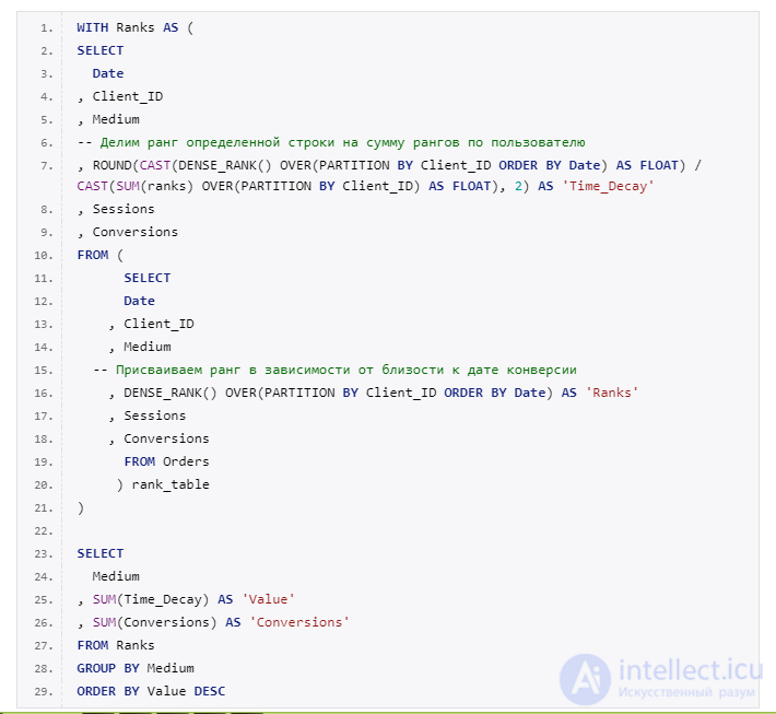
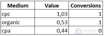
From the resulting report we can see that the most weighty channel is «cpc», while the «cpa» channel, which would have been excluded under the standard attribution model, also received its share when the value was distributed.

In closing

And that's how we broke this dataset down piece by piece using window functions. That wraps up our introduction to window functions. We hope it was interesting and not as complicated as it might have seemed.

Of course, this is far from all the capabilities of window functions. There are many other useful things for them, such as ROWS, NTILE, and aggregate functions (SUM, MAX, MIN, and others), but we'll talk about those another time.

See also

• aggregate function
• scalar function
• query
• subquery