Analysis and Estimation of Algorithm Complexity: Big O and Complexity Functions

Many of today's programmers, who write great and widely used programs, have an extremely vague idea of theoretical computer science. This does not prevent them from remaining excellent, creative specialists, and we are grateful for what they create.

Do you really understand what Big O is? If so, this article will help you refresh your knowledge before an interview. If not, this article will tell you what it is and why you need to know about it.

The Big O notation is one of the most fundamental tools for analyzing algorithm complexity. This article is written on the assumption that you are already a programmer with a substantial amount of written code behind you. In addition, a knowledge of basic high-school mathematics is needed for a better understanding of the material. So, if you're ready, let's begin!

Nevertheless, knowing the theory also has its own advantages and can turn out to be quite useful. In this article, intended for programmers who are good practitioners but have a weak grasp of theory, I will present one of the most pragmatic programming tools: Big O notation and the analysis of algorithm complexity. As someone who has worked both in academic research and in building commercial software, I consider these tools genuinely useful in practice. I hope that after reading this article you will be able to apply them to your own code to make it even better. This post will also bring an understanding of common terms used by computer science theorists, such as «Big O», «asymptotic behavior», «worst-case analysis», and so on.

This text is also aimed at high-school students from Greece or any other country taking part in the International Olympiad in Informatics, algorithm competitions for students, and the like. As such, it does not require knowledge of any mathematical prerequisites and will give you a foundation for further exploration of algorithms with a solid understanding of the theory behind them. As someone who once took part in various competitions a great deal, I strongly recommend that you read and understand the entire introductory material. This knowledge will be simply essential as you go on to study algorithms and various advanced technologies.

I hope that this text will be useful for those practicing programmers who do not have much experience in theoretical computer science (the fact that the most inspired software engineers never went to college is a long-established fact). But since the article is also intended for students, at times it will sound like a textbook. Moreover, some topics may seem overly simple to you (for example, you may have encountered them during your studies). So, if you feel that you understand them — just skip those parts. Other sections go somewhat deeper and are more theoretical, because students taking part in competitions need to understand algorithm theory better than the average practitioner. But knowing these things is no less useful, and following the narrative is not all that difficult, so they probably deserve your attention. The original text was aimed at high-school students, requires no special mathematical knowledge, and so anyone with programming experience (for example, knowing what recursion is) is able to understand it without much difficulty.

In this article you will find many interesting links to material beyond the scope of our discussion. If you are a working programmer, then it is quite possible that you are already familiar with most of these concepts. If you are simply a novice student taking part in competitions, following these links will give you information about other areas of computer science and software development that you have not yet had a chance to study. Look through them to expand your own knowledge base.

Big O notation and the analysis of algorithm complexity are things that both practicing programmers and novice students often find difficult to understand, are afraid of, or simply avoid as useless. But they are not as complicated and abstruse as they may seem at first glance. Algorithm complexity is simply a way to formally measure how fast a program or algorithm runs, which is a very pragmatic goal. Let's start with a bit of motivation on this topic.

Motivation

We already know that there are tools that measure how fast code runs. These are programs called profilers, which determine execution time in milliseconds, helping us identify bottlenecks and optimize them. But, while this is a useful tool, it has nothing to do with algorithm complexity. Algorithm complexity is something based on comparing two algorithms at an ideal level, ignoring low-level details such as the implementation of the programming language, the «hardware» the program is running on, or the instruction set of a given CPU. We want to compare algorithms in terms of what they actually are: ideas about how a computation happens. Counting milliseconds won't help much here. It may well turn out that a bad algorithm written in a low-level language (for example, assembly) will be much faster than a good algorithm written in a high-level programming language (for example, Python or Ruby). So it's time to determine what a «better algorithm» actually means.

An algorithm is a program that represents pure computation, without the other things a computer often does — network tasks or user input/output. Complexity analysis lets us find out how fast this program is when it performs computations. Examples of purely computational operations might include operations on floating-point numbers (addition and multiplication), searching for a given value in an in-memory database, an in-game AI determining how to move its character so that it travels only a short distance within the game world, or running a regular expression pattern match against a string. Clearly, computations occur throughout computer programs.

Complexity analysis also lets us explain how an algorithm will behave as the input data stream grows. If our algorithm runs in one second with 1000 elements as input, how will it behave if we double that value? Will it run just as fast, one and a half times faster, or four times slower? In programming practice such predictions are extremely important. For example, if we've built an algorithm for a web application serving a thousand users and measured its execution time, then using complexity analysis we can get a pretty good idea of what will happen when the number of users grows to two thousand. For algorithm-building competitions, complexity analysis will also give us an understanding of how long our code will take to run on the largest of the tests used to check its correctness. So, if we determine the general behavior of our program on a small amount of input data, we can get a good idea of what will happen with it on large data streams as well. Let's start with a simple example: finding the maximum element in an array.

Counting instructions

In this article I will use various programming languages to implement the examples. Don't worry if you're not familiar with one of them — anyone who knows how to program is able to read this code without much trouble, since it is simple, and I am not going to use any exotic features of the implementation language. If you are a competitive-programming student, you most likely write in C++, so you shouldn't have any problems either. In that case I also recommend working through the exercises using C++ for extra practice.

The maximum element of an array can be found with the simplest snippet of code. For example, one written in Javascript. Given an input array A of size n:

var M = A[ 0 ];

for ( var i = 0; i < n; ++i ) {
    if ( A[ i ] >= M ) {
        M = A[ i ];
    }
}

First let's count how many fundamental instructions are computed here. We'll do this only once — as we go deeper into the theory this need will go away. But for now, be patient with the time we'll spend on it. In analyzing this code, it makes sense to break it down into simple instructions — tasks that can be executed by the processor instantly or nearly so. Suppose that our processor is able to execute the following operations as single instructions:

• Assign a value to a variable
• Find the value of a specific array element
• Compare two values
• Increment a value
• Basic arithmetic operations (for example, addition and multiplication)

We will assume that branching (choosing between the if and else parts of the code after evaluating the if-condition) happens instantly, and we will not count this instruction. For the first line in the code above:

var M = A[ 0 ];

two instructions are required: one to look up A and one to assign the value to M (we assume that n is always at least 1). These two instructions will be required by the algorithm regardless of the value of n. Initialization of the for loop will also occur constantly, giving us two more commands: assignment and comparison.

i = 0;
i < n;

All of this happens before the first run of for. After each new iteration we will have two more instructions: the increment of i and the comparison to check whether it is time to stop the loop.

++i;
i < n;

Thus, if we ignore the contents of the loop body, the number of instructions for this algorithm is 4 + 2n — four for the start of the for loop and two for each iteration, of which we have n. Now we can define a mathematical function f(n) such that, knowing n, we will know the number of instructions the algorithm requires. For a for loop with an empty body, f( n ) = 4 + 2n.

Worst-case analysis

In the body of the loop we have array lookup and comparison operations, which always occur:

if ( A[ i ] >= M ) { ...

But the body of the if may or may not run, depending on the actual value from the array. If it happens that A[ i ] >= M, then two additional commands will run: an array lookup and an assignment:

M = A[ i ]

We can no longer determine f(n) so easily, because now the number of instructions depends not only on n, but also on the specific input values. For example, for A = [ 1, 2, 3, 4 ] the program will need more commands than for A = [ 4, 3, 2, 1 ]. When we analyze algorithms, we most often consider the worst-case scenario. What would that be in our case? When will the algorithm need the most instructions before finishing? Answer: when the array is sorted in increasing order, as, for example, A = [ 1, 2, 3, 4 ]. Then M will be reassigned every time, which gives the largest number of commands. Theorists have a fancy name for this — worst-case analysis, which is nothing other than simply considering the most unfavorable variant. Thus, in the worst case, four instructions run in the loop body of our code, and we have f( n ) = 4 + 2n + 4n = 6n + 4.

Asymptotic behavior

With the function obtained above, we have a very good picture of how fast our algorithm is. However, as I promised, we do not need to constantly engage in such a tedious activity as counting commands in a program. Moreover, the number of instructions a particular processor needs to implement each statement of the programming language used depends on that language's compiler and on the instruction set available to the processor (AMD or Intel Pentium on a personal computer, MIPS on a Playstation 2, and so on). Earlier we said that we intend to ignore conditions of this kind. So now we will pass our function f through a «filter» to clean it of insignificant details that theorists prefer to disregard.

Our function 6n + 4 consists of two elements: 6n and 4. In complexity analysis, what matters is only what happens to the instruction-counting function as n grows significantly. This coincides with the earlier idea of the «worst-case scenario»: we are interested in the behavior of the algorithm under «bad conditions,» when it is forced to do something difficult. Note that this is exactly what is truly useful when comparing algorithms. If one of them beats another on a large input stream of data, there is a good chance it will remain faster on light, small streams too. That is why we discard the elements of the function that grow slowly as n increases, and keep only those that grow strongly. Obviously, 4 will remain 4 regardless of the value of n, while 6n , on the contrary, will grow. So the first thing we do is discard the 4 and keep only f( n ) = 6n.

It makes sense to think of the 4 simply as an «initialization constant.» Different programming languages may need different amounts of time for setup. For example, Java first needs to initialize its virtual machine. And since we have agreed to ignore differences between programming languages, we simply discard this value.

The second thing that can be ignored is the coefficient in front of n. So our function turns into f( n ) = n. As you can see, this simplifies a lot. Once again, it makes sense to discard the constant coefficient if we are thinking about differences in compilation time between different programming languages. «Array lookup» may compile completely differently for one language than for another. For example, in C, performing A[ i ] does not include a check that i does not go beyond the declared array size, whereas for Pascal such a check exists. Thus, the following Pascal code:

M := A[ i ]

is equivalent to the following in C:

if ( i >= 0 && i < n ) {
    M = A[ i ];
}

So it makes sense to expect that different programming languages will be subject to the influence of different factors that will affect the instruction count. In our example, where we use a «dumb» Pascal compiler that ignores optimization possibilities, three instructions are required in Pascal for each array element access instead of one in C. Disregarding this factor is in line with ignoring the differences between specific programming languages, focusing on the analysis of the algorithm's idea itself.

The filters described above — «discard all factors» and «keep only the largest element» — together give what we call asymptotic behavior. For f( n ) = 2n + 8 it will be described by the function f( n ) = n. In mathematical terms, we are interested in the limit of the function f as n tends to infinity. If the meaning of this formal phrase is not entirely clear to you, do not worry — you already know everything you need. (Aside: strictly speaking, in a mathematical formulation we could not discard constants in the limit, but for the purposes of theoretical computer science we do so for the reasons described above). Let us work through a couple of problems to fully grasp this concept.

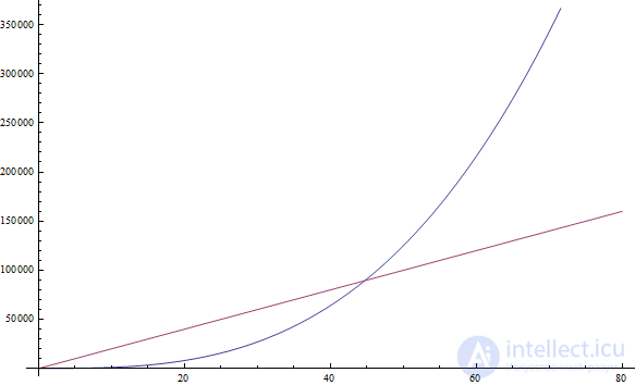
Let us find the asymptotics for the following examples, using the principles of discarding constant factors and keeping only the fastest-growing element:

1. f( n ) = 5n + 12 gives f( n ) = n.
   The reasons are the same as described above
2. f( n ) = 109 gives f( n ) = 1.
   We discard the factor in 109 * 1 , but the 1 is still needed to show that the function is not zero
3. f( n ) = n² + 3n + 112 gives f( n ) = n²
   Here n² grows faster than 3n, which in turn grows faster than 112
4. f( n ) = n³ + 1999n + 1337 gives f( n ) = n³
   Despite the large magnitude of the coefficient in front of n, we still assume that we can find an even larger n, so f( n ) = n³ is still greater than 1999n (see the figure above)
5. f( n ) = n + sqrt( n ) gives f( n ) = n
   Because n grows faster than sqrt( n ) as the argument increases