
Lecture
In the previous lectures we studied various aspects of data warehouse (DW) logical design methods. Logical design methods are based on an abstract treatment of data. A logical model is in no way tied to a specific implementation of the model in a DBMS database.
In practice, DWs are created and operated as databases managed by a specific DBMS. Databases implementing a DW are built on the basis of a physical data model developed by the DW designer and implemented as database objects.
A physical data model, by contrast, depends on the specific DBMS and contains information about all the objects of the database. Since there are no standards for database objects (for example, there is no standard for data types), the physical model depends on the specific DBMS implementation and its dialect of SQL. Consequently, one and the same logical data model may correspond to several different physical models.
The main objects of a logical data model are entities, attributes, and relationships. A physical data model is, as a rule, built on the basis of the logical one, so each object of the logical model corresponds to an object of the physical model (although the correspondence may be ambiguous). In the physical data model, an entity of the logical data model corresponds to a table, an instance of an entity corresponds to a row in the table, and an attribute corresponds to a column of the table. In addition to the objects listed above, a physical model may contain objects whose type depends on the DBMS: indexes, views, sequences, triggers, stored procedures, and so on. Whereas in a logical data model it is not very important which specific data type an attribute has, in a physical model it is important to describe all the information about specific objects.
Further on, when presenting the material, we will assume that we are dealing with relational or object-relational DBMSs and their corresponding SQL dialects.
Two stages can be distinguished in creating a physical data model [48]. The main goals of the first stage are:
At the first stage, within the requirements of the relational model, data storage objects are created that correspond to the entities and relationships of the logical data model — tables, indexes, views, and so on.
The main goal of the second stage is to ensure the required level of performance. To achieve this goal, one must take into account both the implementation features of the DBMS for which the physical model is being created and the operating characteristics of the future information system as a whole. Database performance is usually measured in terms of transaction performance.
To improve transaction performance, objects created at the first stage may be modified, or new database objects may be created. In other words, developing a physical model is an iterative process, and there may be several iterations (create objects – analyze transactions – modify objects – analyze transactions). Issues of improving transaction performance will be covered in one of the following lectures.
One of the main tasks that the designer must solve at the stage of designing the physical model of a DW is turning objects of the logical data model into objects of a relational database. To solve this task, the designer needs to know: a) what objects a relational database has in principle; b) which objects are supported by the specific DBMS chosen for implementing the database.
Thus, we assume that the decision on choosing the DBMS has already been made by the IT project manager and agreed with the customer of the database, i.e., the DBMS is given. The DW designer must become familiar with the documentation describing the SQL dialect supported by the chosen DBMS. In this lecture it is assumed that a DBMS from the MS SQL Server family from Microsoft has been chosen, although the overwhelming majority of the material covers objects in any industrial-grade relational DBMS.
The hierarchy of relational database objects is set out in the SQL standards, in particular in the SQL-92 standard, which we will use as a guide when presenting the material of this lecture. This standard is supported by practically all modern DBMSs. The hierarchy of database objects is shown in Fig. 11.1.
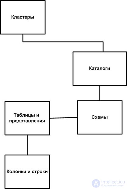
At the lowest level are the objects that the relational database works with — columns and rows. These, in turn, are grouped into tables and views. Note that in the context of the lecture the terms attribute, column, and field are considered synonyms. The same applies to the terms "row," "record," and "tuple."
Tables and views, which represent the physical reflection of the logical structure of the database, are grouped into a schema. Several schemas are grouped into catalogs, which can then be grouped into clusters.
It should be noted that none of the groups of objects in the SQL-92 standard is tied to the physical structures used for storing information in computer memory.
In addition to the objects shown in the figure, a relational database may also have indexes, triggers, events, stored commands, stored procedures, and a number of others. Let us now move on to defining the database objects.
Clusters, catalogs, and schemas are not mandatory elements of the standard and, consequently, of the database software environment.
A cluster is understood as a group of catalogs that can be accessed through a single connection to the database server (a software component of the DBMS).
Usually the procedure for creating a catalog is defined by the DBMS implementation on a specific operating platform. A catalog is understood as a group of schemas. In practice, a catalog is often associated with a physical database as a set of operating-system physical files identified by its name.
For a database designer, a schema is a general logical representation of the relations of a complete database. From an SQL point of view, a schema is a container for tables, views, and other structural elements of a relational database. The principle for placing database elements within each schema is entirely determined by the designer. In practice, a schema is often associated with the objects of a particular user — the owner of the physical database.
Below, database objects will be defined in the context of MS SQL Server 2005/2008. This approach is taken because designing a physical database model is done for a specific implementation environment.
On MS SQL Server 2005, a schema (Schema) is a collection of database objects — tables, views, stored procedures, triggers — forming a single namespace. Schemas and users are different objects of the physical database. Each schema has an owner — a user, or a role (see below).
The main objects of relational databases include the table, the view, and the user.
A table (Table) is the basic structure of a relational database. It represents a unit of data storage — a relation. A table is a two-dimensional array of data in which the column defines the value and the rows contain the data. A table is identified in the database by its unique name, which includes identification of the user. A table can be empty or consist of a set of rows.
A view (View) — is a named selection, dynamically maintained by the DBMS, from one or more tables of the database. The selection statement limits the data visible to the user. Usually the DBMS guarantees that the view is up to date: it is generated each time the view is used. Views are sometimes called virtual tables.
A user (User) — is an object that has the ability to create or use other database objects and to request the execution of DBMS functions, such as establishing a session, changing the state of the database, and so on.
To simplify the identification and naming of objects, the database supports such objects as the synonym, the sequence, and user-defined data types.
A synonym (Synonym) — is an alternative name (alias) for a relational database object that allows access to that object. A synonym can be public or private. A public synonym allows all database users to access the corresponding object by its alias. A synonym allows the full qualification of an object in the database to be hidden from end users.
User-defined data types (User-defined data types) are user-defined attribute types (domains) that differ from the types supported (built in) by the DBMS. They are defined on the basis of the built-in types.
Rules (Rules) – are declarative expressions that restrict the possible values of data. Rules are formulated using valid SQL predicate expressions.
To ensure efficient access to data, relational DBMSs support a number of other objects: the index, the tablespace, the cluster, the partition.
An index (Index) — is a database object created to improve the performance of data retrieval and to control the uniqueness of the primary key (if one is defined for the table).
A partition (Partition) — is a database object that allows an object with data to be represented as a set of sub-objects assigned to different tablespaces. Thus, partitioning allows very large tables to be distributed across several hard disks.
To process data in a special way or to implement support for referential integrity of the database, the following objects are used: the stored procedure, the function, the command, the trigger. These database objects can be used to perform so-called row-by-row processing (record processing) of data. From the point of view of database applications, row-by-row processing means sequentially fetching data one row at a time, processing it, and moving on to processing the next row.
These objects of a relational database are programs, i.e., executable code. This code is usually called server-side code, since it is executed on the computer on which the relational DBMS engine is installed. Planning and developing such code is one of the tasks of a relational database designer.
A stored procedure (Stored procedure) — is a database object representing a named set of SQL commands and/or statements of specialized database programming languages.
A function (Function) — is a database object representing a named set of SQL commands and/or statements of specialized database programming languages, which, when executed, returns a value — the result of the computation.
A trigger (Trigger) — is a database object that is a special kind of stored procedure. This procedure runs automatically when an event associated with the trigger occurs (for example, inserting a row into a table).
For efficient management of access control, the role object is supported.
A role (Role) – a database object representing a named set of privileges that can be assigned to users, categories of users, or other roles.
In the logical data model, the implementation environment is not taken into account. It defines attributes and their possible values, such as string, number, or date; ideally, an attribute can be assigned a domain. A domain is simply the type of an attribute, for example, "Money" or "Business day." The designer may include a number of validity checks or processing rules, for example, a requirement that a value must be positive, nonzero, and have at most two decimal places (which is useful for computing the amounts of ruble payments a bank charges to another bank).
Using domains simplifies the task of ensuring consistency at the logical data model stage. When moving on to designing the physical data model, the designer needs to know the capabilities of the chosen DBMS for assigning column data types. In the logical data model, the values that a relation's attribute may take are also specified by a domain, which is inherited from the information model. In the physical database model, each relation attribute in the database is required to have a number of properties that dictate what can and cannot be stored in it. These properties are the type, size, and constraints, which may further restrict the allowed set of values of the column. The task is to convert the domain into a suitable data type supported by the DBMS. Thus, the designer must know which data types are available when solving the above task.
In the context of designing the physical model of a relational database, a domain is an expression that defines the allowed values for the columns (attributes) of a relation. When describing a table of a relational database, each column is assigned a specific data type. In practice, the data type contained in a column forms the basis for defining the domain, since most built-in types specify an allowed interval of data values.
Example 11.1. A column in a database can be described as follows:
amount NUMBER (8,2) NOT NULL CONSTRAINT cc_limit_amnt CHECK
(amount > 0)
The column "Payment amount" ( Amount ) can only hold numeric data; its precision is two significant decimal places ( NUMBER (8,2) ); it must be filled in for every row of the table ( NOT NULL ); its value must be positive CONSTRAINT cc_limit_amnt CHECK (amount > 0). The maximum value that can be stored in this column is 999999.99. In this simple column definition we have in fact defined a number of implicit rules, the checking of which MS SQL Server forcibly enables when data is entered into the database.
As we can see, further defining a column's domain (after assigning it a type) is done by the designer by refining the rules for changing values. Such refinements are supported in SQL through the constraint mechanism in a table's column specification.
The SQL-92 standard introduced the concept of user-defined domains. The definition of such domains is based on the DBMS's built-in data types.
A data type is a specification defining what kind of data can be stored in a database object: integers, characters, monetary data, timestamps and dates, binary strings, and so on.
All allowed data types are described in the SQL-92 standard, but most dialects support an extended list of data types. However, any SQL dialect supports three general data types: string, numeric, and a type for representing date and time. Specifying a data type determines the values and length of the data, as well as the format in which it is displayed.
For every data type there is a so-called null value, which indicates the absence of data in a column of the specified type, i.e., the fact that the data value is currently unknown.
The description of the types given in the table below relates to the SQL dialect of the MS SQL Server family of DBMSs, which has significant differences from the requirements of the SQL standard. The part of a reserved word for defining a type that can be used as an abbreviation when defining the type in a column specification is shown in bold.
MS SQL Server provides a set of system data types that define all the data types that can be used in it. You can also define your own data types in Transact-SQL or the Microsoft .NET Framework. Data type aliases are based on system types. User-defined data types have properties that depend on the methods and operators of the class created for them in one of the programming languages supported by the .NET Framework.
When two expressions with different data types, collations, precisions, scales, or lengths are combined by an operator, the result is determined as follows.
Data types in the MS SQL Server family of DBMSs are grouped into the following categories:
| Data type | Syntax |
|---|---|
| Exact numbers | |
| bigint | Integer values in the range from  to to  |
| int | Integer values in the range from  to to  |
| smallint | Integer values in the range from  to to  |
| tinyint | Integer values in the range from 0 to 255 |
| bit | An integer equal to 1, 0, or NULL |
| decimal[ (p[ , s] )] and numeric[ (p[ , s] )] | Fixed-precision, fixed-scale numbers. At maximum precision, the numbers can take values in the range from  to to  . .
p (precision) – the maximum total number of decimal digits in the number (both to the left and to the right of the decimal point). Precision must take a value from 1 to 38. The default precision value is 18. s (scale) – the maximum number of decimal digits to the right of the decimal point. Scale can take a value from 0 to p. Scale can only be specified together with precision. By default, scale is 0, so 0 <= s <= p. The maximum storage size depends on the precision. |
| money | Monetary (currency) values in the range from -922,337,203,685,477.5808 to 922,337,203,685,477.5807 |
| smallmoney | Monetary (currency) values in the range from -214,748.3648 to 214,748.3647 |
| Approximate numbers | |
| float
float [ ( n ) ] |
Floating-point numeric values in the ranges:  - -  and and  - -  . .
n is the number of bits used to store the mantissa of a float number in exponential notation, which determines the precision of the data and the storage size. The value of the n parameter must lie between 1 and 53. The default value of the n parameter is 53 |
| real | Floating-point numeric values in the ranges:  - -  and and  - -  |
| Date and time | |
| date | A date in YYYY-MM-DD format. Range of values from 0001-01-01 to 9999-12-31, from January 1, year 1, to December 31, year 9999 |
| datetime | Defines a date combined with a time of day, including fractions of a second, in 24-hour format, from January 1, 1753 to December 31, 9999, from 00:00:00 to 23:59:59.997 |
| smalldatetime | Defines a date combined with a time of day. The time is represented in 24-hour format with seconds always equal to zero (:00), without fractions of a second, from 01/01/1900 to 06/06/2079, January 1, 1900 to June 6, 2079, from 00:00:00 to 23:59:59 |
| time | Defines a time of day. Time without time-zone awareness in 24-hour format, from 00:00:00.0000000 to 23:59:59.9999999 |
| datetime2 | Defines a date combined with a time of day in 24-hour format. From 0001-01-01 to 9999-12-31, from January 1, year 1 AD, to December 31, year 9999 AD, from 00:00:00 to 23:59:59.9999999 |
| datetimeoffset | Defines a date combined with a time of day, with time-zone awareness, in 24-hour format, from 0001-01-01 to 9999-12-31, from January 1, year 1 AD, to December 31, year 9999 AD, from 00:00:00 to 23:59:59.9999999 |
| Character strings | |
| varchar [( n| max )] | Variable-length, non-Unicode character data. n can be a value from 1 to 8,000; max means the maximum storage size is bytes. The storage size equals the actual length of the data plus two bytes. The entered data can be 0 characters long. The ISO standard synonyms for the varchar type are char varying or character varying |
| char [ ( n ) ] | Fixed-length, non-Unicode character data with a length of n bytes. The value of n must be in the range from 1 to 8000. The storage size for data of this type equals n bytes. The ISO standard synonym for the char type is character |
| text | This data type represents non-Unicode data using the server's code page. The maximum data length is  - 1 (2,147,483,647) characters. If the server's code page uses double-byte characters, the space occupied by the type still does not exceed 2,147,483,647 bytes. It may be less than 2,147,483,647 bytes, depending on the character string - 1 (2,147,483,647) characters. If the server's code page uses double-byte characters, the space occupied by the type still does not exceed 2,147,483,647 bytes. It may be less than 2,147,483,647 bytes, depending on the character string |
| Unicode character strings | |
| nchar [ ( n ) ] | Unicode character data of length n characters. The argument n must have a value from 1 to 4000. The storage size is twice n bytes. The ISO standard synonyms for the nchar type are national char and national character |
| nvarchar [(n|max )] | Variable-length Unicode character data. The argument n can take a value from 1 to 4,000. The argument max indicates that the maximum storage size is bytes. The storage size in bytes is twice the number of characters entered, plus 2 bytes. The entered data can be 0 characters long. The ISO standard synonyms for the nvarchar type are national char varying and national character varying |
| ntext | This data type represents variable-length Unicode character data, containing up to  - 1 (1,073,741,823) characters. The space occupied by this type (in bytes) is twice the number of characters. In the SQL-2003 specification, the synonym for the ntext data type is national text - 1 (1,073,741,823) characters. The space occupied by this type (in bytes) is twice the number of characters. In the SQL-2003 specification, the synonym for the ntext data type is national text |
| Binary data | |
| binary [ ( n ) ] | Fixed-length binary data of size n bytes, where n is a value from 1 to 8000. The storage size is n bytes |
| varbinary [(n|max)] | Variable-length binary data. n can be a value from 1 to 8000; max means the maximum storage length, which is bytes. The storage size is the actual length of the entered data plus 2 bytes. The entered data can be 0 characters in size. In SQL-2003 the synonym for varbinary is binary varying |
| image | This type represents variable-length binary data, containing from 0 to - 1 (2,147,483,647) bytes |
| Other data types | |
| timestamp | This is a data type that represents automatically generated unique binary numbers within a database. The timestamp data type is used mainly as a mechanism for versioning table rows. The storage size is 8 bytes. The timestamp data type is merely an increasing value that does not store a date or time. The datetime data type is used to record a date or time |
| xml ([CONTENT| DOCUMENT] xml_schema_collection ) | A data type used to store XML data. You can store xml instances in a column or in a variable of type xml.
CONTENT. The xml instance must be a well-formed XML fragment. XML data can contain several (0 or more) top-level elements. Text nodes are allowed at the top level. This is the default behavior. DOCUMENT. The xml instance must be a well-formed XML document. The XML data must contain only one root element. Text nodes at the top level are not allowed. xml_schema_collection. The name of the XML schema collection. To create a typed xml column or variable, you can additionally specify the name of the XML schema collection. Additional information on typed and untyped XML |
| sql_variant | A column of type sql_variant can contain values of different data types. For example, a column defined as sql_variant can store int, binary, and char values |
| table | A special data type that can be used to store a result set for subsequent processing. The table type is used mainly for temporarily storing a set of rows returned as the result set of a table-valued function |
| cursor | A data type for variables or output parameters of stored procedures that hold a reference to a cursor. Any variable created with the cursor data type can take the value NULL |
So, we have looked at the main database objects and the allowed data types available to the DW designer when using a DBMS from the MS SQL Server family.
Next, let us talk about the algorithm for creating a physical DW model.
As an example, let us consider the "star" logical DW model in Fig. 11.2 and build a physical DW model on its basis.
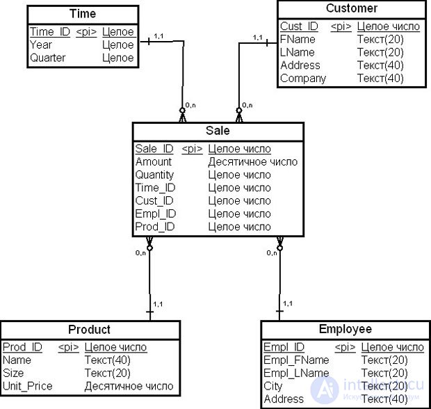
The logical model of the data warehouse shown in the figure was developed to analyze the company's sales broken down by products, salespeople, customers, and sales time. It includes four dimension entities: "Time", "Customer", "Product", "Employee" (salesperson) – and one fact entity, "Sale".
As the diagram shows, the domains defined for the attributes are "Integer", "Decimal number", and "Text" of 20 and 40 characters in length.
A description of the model's attributes is given in Table 11.2.
| Attribute | Value | Entity |
|---|---|---|
| Time_ID | Time identifier, entity key | "Time" |
| Year | Year | "Time" |
| Quarter | Quarter of the year | "Time" |
| Cust_ID | Customer identifier, entity key | "Customer" |
| FName | Customer's first name | "Customer" |
| LName | Customer's last name | "Customer" |
| Address | Customer's address | "Customer" |
| Company | Place of employment | "Customer" |
| Prod_ID | Product identifier, entity key | "Product" |
| Name | Product name | "Product" |
| Size | Product dimensions | "Product" |
| Unit_Price | Price per unit of product | "Product" |
| Empl_ID | Salesperson identifier, entity key | "Employee" |
| Empl_FName | Salesperson's first name | "Employee" |
| Empl_LName | Salesperson's last name | "Employee" |
| City | City/locality | "Employee" |
| Address | Location address | "Employee" |
| Sale_ID | Sale identifier, entity key | "Sale" |
| Amount | Payment amount | "Sale" |
| Quantity | Quantity | "Sale" |
After reviewing the documents describing the logical model of the data warehouse, the designer's next task is to build the physical model of the data warehouse, which includes the following steps.
продолжение следует...
Часть 1 The physical model of a data warehouse
Часть 2 Developing a script for creating the objects of the data
Часть 3 Constraints and their use in a relational database - The
Часть 4 Summary - The physical model of a data warehouse

Comments