
Lecture
Before discussing the main types of database applications, let us clarify the terms transaction and query. In database theory, generally speaking, a transaction is understood as one of the SQL commands — SELECT, INSERT, UPDATE, DELETE. However, depending on the type of application, the term "transaction" is interpreted more loosely, as an elementary, logically complete unit of work (the so-called business transaction), which may include several insert, delete, or modify commands. Depending on which SQL commands are used, transactions are divided into insert-only (write-only), modify-only, read-only, and delete-only transactions. Read-only transactions are called queries.
Based on this division of transactions by processing type, together with the frequency of transactions of each type, we can identify three main classical types of database applications.
A few more types of applications can be identified that have appeared over the last two decades.
To analyze transactions, it is necessary to assess the type of application for which the database is being developed. This makes it possible to estimate:
Recall that a database transaction is a logical unit of work that transforms the database from one complete state to another complete state. Here, a complete state of the database is understood as a state that does not violate the integrity of the data, when all data in the database tables is correct and the references between tables are consistent. In addition, a transaction groups operations on data in such a way that either all accesses to the database are completed successfully, or, in case of failure, the database is returned to the previous complete state (transaction rollback).
Since any data-modification operation in a database carries the potential to violate data integrity, it is necessary to strictly define transactions and identify the information that is normally included in a transaction definition.
A transaction definition can take various forms. Sometimes the data repository of a database-design CASE tool is used to define transactions. Very often, transaction definitions are produced by means of textual descriptions. Regardless of the chosen approach, any good transaction definition includes several important elements. These elements include:
The first step in defining transactions is uniquely identifying each database transaction. This can be done by assigning a name and a number to each database transaction. Transaction names should let users distinguish them from one another. The description includes a list of domain operations that the transaction performs. It should be written in terms of the subject domain that are understandable to the user. Here the following should be kept in mind:
Example 19.1. Transaction description.
Transaction name: assign a job to an employee.
Transaction description. The transaction checks whether this job has already been assigned to this employee, then checks whether the employee has available working time to perform this job. If the results of the checks are positive (the job has not been assigned to this employee, and the employee has time available to perform it), then the job is assigned to the employee.
In OLTP systems, most transactions are known in advance, so there is a one-to-one correspondence between the transaction specification and the database transaction. In DSS systems, transactions are often unknown in advance, and consequently it is fundamentally impossible to describe all of them. In this case, the specification only describes database transactions in general terms, so it is important to be able to predict the type of transactions that a user is most likely to perform against the database.
For each transaction, the nature of the transaction can be defined (online transaction or batch transaction), and its complexity can be indicated as well. Complexity is usually specified in terms of "high," "medium," "low." This information is needed to assess the database transactions as a whole. The number of transactions of a given complexity affects the time required to design the physical model of the database: the more high-complexity transactions there are in the database, the longer the physical model design takes. Transaction complexity is a conventional measure of the effort involved in meeting the database's performance requirements.
High complexity is usually assigned to a transaction that has two of the following characteristics:
Low complexity is assigned to a transaction with the following characteristics:
A transaction of medium complexity has characteristics between low and high complexity.
Example 19.2. Defining transaction characteristics.
Nature of the transaction: online transaction.
Complexity: medium.
Information about transaction frequencies usually includes two parameters — the average transaction frequency (for example, 50 transactions/hour) and the peak transaction frequency (for example, 70 transactions/hour). Estimating the frequency characteristics of the database is very important for designing the physical data model of a data warehouse: tuning the physical structure of the database for high-frequency transactions differs substantially from tuning it for low-frequency transactions.
Example 19.3.
Average transaction frequency: up to 10 per day.
Peak frequency: 10 per hour.
While for modernizing existing systems, information on transaction frequencies can be provided in the input documentation based on an analysis of operational statistics, for a data warehouse being newly created, obtaining such information is practically impossible, and one has to rely on rough estimates.
The transaction specification should include performance requirements. The overall performance of a database is made up of the performance of each individual transaction and their distribution over time. This is very important information for solving the problem of tuning the physical structure of the data warehouse. Performance requirements are usually specified as a response time parameter, i.e., the number of seconds required to execute the transaction. For example, in many banking systems a transaction for withdrawing money from a customer's account must not take more than 5 seconds.
Another way of specifying performance requirements for database transactions is to indicate their nature and complexity. For example,
Obtaining performance requirements for transactions is one of the biggest bottlenecks both in the source documentation and in the physical design of the data warehouse model. In practice, the timing characteristics of transaction execution can often only be obtained at the pilot-operation stage, or even during the production operation of the data warehouse.
It is desirable for the transaction specification to indicate its relative priority, which shows how important this particular transaction is for the subject domain compared to others. Relative priority allows transactions to be grouped by this parameter, making it possible to consistently evaluate all database transactions and their contribution to database performance.
Executing some transaction in the database with a high priority has a negative effect on the performance of other transactions. Ranking by relative priority makes it possible to balance the overall mutual influence of transactions on one another.
Assigning transaction priority can take various forms. Usually this comes down to a subjective rating expressed as a number from 1 to 10.
Every transaction specification should contain the SQL commands that define the database operations. Specifying the SQL commands in the context of building the physical model of the data warehouse makes it possible to estimate the transaction execution time (execution time), i.e., the actual number of seconds needed to complete the transaction while the data warehouse is in operation. This parameter is also important for the data warehouse designer from the standpoint of writing specifications of the data warehouse's application modules for application developers.
In addition to the actual data-manipulation-language command, it is advisable to include a comment for each command indicating: a) what the command does, b) why it is required, and c) the number of rows in the data warehouse affected by the command. The execution time of an SQL command directly depends on the number of rows processed by the command. Usually the execution time of transactions can be estimated at the pilot-operation and database-testing stage.
Example 19.4.
| Command | Comment |
|---|---|
| Select works from project where empno=:1 and works=:2 | Returns information about the assignment of this job to this employee. At least one row is returned. The number of rows that the command may process is equal to the current size of the PROJECT table |
| Select works from project where empno=:1 | Returns the list of jobs for this employee, in order to assess his workload. The number of rows that the command may process is equal to the current size of the PROJECT table |
| Insert into project empno, works values(:1, :2) | Assigns this employee to this job, if needed |
A description of transactions makes it possible to decide whether to make or defer a decision on changing the physical schema of the data warehouse in order to meet database performance requirements.
The mechanisms by which performance requirements can be met are discussed below, on the assumption that a DBMS from the MS SQL Server family has been chosen for building the data warehouse, except for one example, which uses the SQL dialect of a DBMS from the Oracle family.
Starting with this section, we will look at techniques for tuning the physical structure of the relational database used to implement the data warehouse, in order to meet the data warehouse's performance requirements. These techniques constitute a set of recommendations and heuristic rules for changing the physical structure of the database that resulted from the first iteration of building the physical data model of the data warehouse. It is clear that applying these techniques is advisory in nature.
In this section we will describe various types of denormalization and methods for implementing it. In addition, we will examine how, when performing denormalization, data integrity can be ensured without resorting to writing additional code.
Denormalization is understood as the process of reaching trade-offs in normalized tables by deliberately introducing redundancy in order to increase performance.
In most cases, the need for denormalization becomes evident only at the stage of designing data warehouse applications or during their operation. In other words, a decision on denormalization cannot be made on the basis of the data model alone. Usually one tries to identify critical processes in the data warehouse's applications and make denormalization decisions primarily in favor of these processes. Critical processes are typically identified by high frequency, large volume, high volatility, or explicit priority. A high-quality description of database transactions makes it possible to identify the presence of such critical processes.
Note that applying denormalization merely to simplify SQL queries when accessing the data warehouse is the wrong decision. If you want to simplify SQL queries at the application or user level, it is probably better to use views rather than introduce redundancy. To improve query performance, indexes can be introduced instead.
As a rule, denormalization reduces query time at the expense of DML operations. Denormalization should be viewed as an extension of the normalized data model that improves query performance. When deciding on denormalization, one should determine what is most important for the application — data redundancy or high performance. If a design log is kept (some free-form internal document in which all decisions made during the data warehouse design process are recorded), then the reasoned decision on denormalization must be entered into it. It should be remembered that, besides denormalization, there are other ways to improve performance. Table denormalization can be performed both at the logical data model level and at the physical model level.
Let us look at the principles of denormalization at the physical data model level. Downward denormalization involves moving a column from one (parent) table into a subordinate (child) table.
Figure 19.1 shows two tables – "Customer" (Customer befor) and "Order" (Order befor) – of the physical data model before denormalization, and Figure 19.2 shows the same tables, "Customer" (Customer after) and "Order" (Order after), after downward denormalization has been performed.

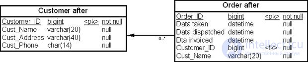
From the figures we can see that in the denormalized model we moved the column "Customer Last Name" (Cust_Name) from the "Customer" (Customer after) table into the "Order" (Order after) table.
What does introducing this redundancy (moving the column) give us in this case? The only benefit is that we eliminate the join operation if we want to see the customer's last name together with the order.
Thus, downward denormalization is the process of introducing redundant columns in child tables in order to eliminate join operations.
However, eliminating joins by means of downward denormalization rarely justifies the cost of maintaining a duplicate column in the "Order" table. Such joins, as a rule, are not a major problem, while performing downward denormalization can lead to expensive cascading updates. For example, if a customer changes their last name, all orders must be updated to reflect this change. But is that really necessary? Should old orders that have been completed or closed be updated? Had denormalization not been performed, these questions would never have arisen.
Downward denormalization is justified only in applications where join operations between tables must be eliminated. This is the case in large-volume data warehouses. Here there is no problem with cascading updates, because the data in the data warehouse has the property of stability, i.e., it does not change once it has been loaded into the data warehouse.
Upward denormalization involves moving a column from a subordinate (child) table into the parent table, usually in the form of summary data.
Figure 19.3 shows two tables – "Order" (Order befor) and "Order Item" (Order item befor) – of the physical data model before denormalization, and Figure 19.4 shows the same tables, "Order" (Order after) and "Order Item" (Order item after), after upward denormalization has been performed.
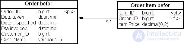
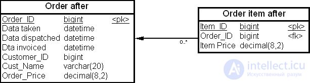
For example, if computing the total order amount in an order-processing system (summing the "Item Price" (Item_Price) column in the "Order Item" table) causes a performance degradation, we can improve the performance of this operation by placing the order total in a redundant "Order Amount" (Order Price) column of the "Order" (Order after) table.
In our example the redundant column stores a sum of values, but upward denormalization is also applicable to maximum, minimum, and average values, as well as other aggregate measures.
Thus, upward denormalization is the process of introducing redundant columns in parent tables in order to eliminate joins combined with aggregation operations.
To illustrate the consequences of introducing denormalization, let us look at the procedure for maintaining the denormalized "Order" (Order after) and "Order Item" (Order item after) tables, which comes down to enforcing the following business rules.
Maintaining the business rules listed above creates additional load on the processes that perform DML operations on the "Order Item" (Order item after) table. This is precisely the price that has to be paid for improved query performance.
Intratable denormalization is performed within a single table, i.e., it is the process of introducing redundant columns in one table in order to increase the performance of retrieving a row by a derived value. For example, if a row contains two numeric columns, X and Y, then the value Z, equal to the product of X and Y (Z=X*Y), is easy to compute at run time.
Suppose there are queries that need to search by Z (for example, Z falls in the range from 10 to 20). By storing the redundant values of Z in a column, an index on Z can be built, and queries will use this index. If an index on Z is not needed, then the decision on whether to store it in a separate column depends on which is more acceptable — the increase in load time caused by the need to constantly recompute Z, or the increase in scan time caused by the lengthening of table rows due to storing the additional column.
Let us give one more commonly encountered example of intratable denormalization. Suppose the same text is stored in two forms: with mixed upper and lower case characters — for display in reports and on screen, and with characters all in upper case — to support fast case-insensitive queries.
Note that acceptable performance for moderately sized tables (up to 10,000 rows) can, in the latter case, be achieved without intratable denormalization by rewriting the query using the built-in UPPER function.
Intratable denormalization is rarely used when designing a data warehouse.
Denormalization by the "divide and conquer" method – is the process of splitting a normalized table into two or more tables and creating a one-to-one relationship between them, in order to eliminate additional I/O operations or for technical reasons.
Using this technique is usually driven by technical reasons. As a rule, this method is applied to denormalize tables containing columns with data of type text or varbinary (max), whose size may be 64K or more.
Sometimes it is better to move such a column out into a separate table. Consider a table whose rows contain key columns first, then non-key columns, and finally a column of type varbinary (max). Suppose that in most rows the varbinary (max) column contains data. If there are no indexes on the non-key columns, then when executing queries on any of these columns the DBMS will typically perform a full table scan. In doing so, because the table contains a column of type varbinary (max), additional I/O operations will be required.
To eliminate this problem, the table must be split as shown in Figure 19.5.

In some DBMSs a table cannot have more than 254 columns, and if a table with a larger number of columns is needed to represent the data, this too becomes a reason to split such a table into two. As a rule, such tables arise in the following cases:
According to a well-known specialist in relational database design, D. Ensor, "a good measure of the degree of normalization is the number of columns per table. The rule of thumb states that "very few primary keys have more than twenty attributes that are truly dependent on them."
Denormalization by the table-merging method – is the process of combining two or more normalized tables in order to eliminate join operations or, in some cases, to reduce the number of insert operations.
A reasonable question arises: why, after so much effort has gone into normalizing data structures and splitting entities apart, would one now propose merging tables back together? In fact, merging is justified only in very few cases.
One example of a well-justified use of merging is the presence of a repeating group that is guaranteed to consist of a fixed number of elements. Good candidates for such a merge are tables with a row for each month of the year or each day of the week. The only case in which fixed groups are reliable is when they correspond to absolutely constant things, such as days of the week.
Whether such a merge will actually provide any benefit is hard to say in advance. The approach to denormalization must be determined by the data-processing requirements.
An alternative to this method of denormalization is physically placing tables in a database cluster (as, for example, in DBMSs of the Oracle family). This makes it possible to store the rows of logically related separate tables close together.
Thus, in practice denormalization represents a set of techniques for transforming tables in order to improve query-processing performance. From the standpoint of relational theory, we are, so to speak, disregarding the extraction of certain functional dependencies into separate entity tables. The main criterion for denormalizing normalized tables is the data-processing requirements. In relational databases, unwarranted table denormalization should be avoided.
Table partitioning (splitting partition) is one of the general denormalization methods used in the physical design of a data warehouse. Table partitioning comes in two kinds – vertical partitioning and horizontal partitioning.
Vertical partitioning (vertically partition) is the process of moving some of a table's columns into another, new table that has the same primary key as the source table.
Horizontal partitioning (horizontally partition) is the process of moving some of a table's rows into another, new table that has the same internal structure as the source table.
The main reasons for partitioning a table are either that certain query-performance problems exist on that table, or that disjoint subsets of the table's rows differ significantly in processing performance, i.e., the subsets of rows rarely occur together in the same query.
Query performance problems on tables with long rows are the most common reason for performing vertical table partitioning. The criteria for considering a row to be long may include the following:
Let us consider the case where the row length exceeds the size of the DB's physical page. Here, either the table has too many columns, or some columns have a large length. In this case, when inserting a row into the table, the DBMS will use one or more additional physical pages to store the row. Consequently, retrieving the row from the table will require more I/O operations, proportional to the number of additional physical pages. Query performance will therefore degrade. To increase retrieval performance, the table can be split into one or several tables with a suitably sized row length.
The vertical partitioning method is fundamentally simple if we recall that partitioning is equivalent to the relational projection operation on the table. It is clear that some columns are simply moved into the new table so that the length of the remaining row becomes suitable (< 1 KB). Partitioning must not violate functional dependencies between columns. Since we assume that the original table is normalized (in particular, all non-key columns are fully functionally dependent on the primary key), the primary key of the new table is an exact copy of the primary key of the original table.
A critical question is which columns should be moved into the new table. When a table is partitioned, the performance gain is achieved only when the resulting tables are accessed separately. When the resulting tables are joined, the performance of such a query may be lower than for the same query against the original table, due to the additional I/O. Therefore, before deciding to partition a table, it is necessary to analyze all high-priority transactions against the original table and, when distributing columns among the tables, follow the principle that the frequency of joint use of the columns placed in each partitioned table in queries should be sufficiently high.
Example 19.5.
Suppose that in the "Employees" (EMPLOYEE) table it is necessary to additionally store an employee's photo and biography (fig. 19.6). These two new fields are quite large, and the row length of the table will almost certainly exceed 1 KB.
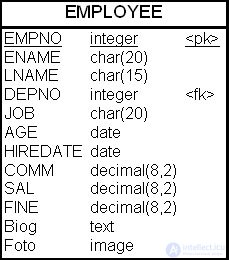
Further, suppose there are 60 transactions that access this table. Only four of them access all columns: entering employee data on hire, making changes, deleting employee information upon termination, and a manager's query, which has high priority. All transactions except the one mentioned above have medium or low priority. The high-priority transaction is expected to occur no more than twice a week. Therefore, splitting the table into two will not significantly affect the performance of high-priority transactions in the database as a
продолжение следует...
Часть 1 The physical model of a data warehouse: accounting for the impact of transactions, table denormalization
Часть 2 Column denormalization - The physical model of a data warehouse:

Comments