
Lecture
SQL – is a data manipulation language for a relational database. In this lecture we will focus on the capabilities that SQL provides for analytical work in a data warehouse.
The only means of communication with a relational database for database administrators, designers, developers, and users alike is the structured query language SQL (Structured Query Language). SQL is a full-featured data manipulation language for relational databases. It is now the universally recognized, standard interface for relational databases such as Oracle, Sybase, DB/2, MS SQL Server, and a number of others (ANSI and ISO standards).
SQL — is a non-procedural language designed for processing sets consisting of the rows and columns of relational database tables. Extensions to SQL exist that allow procedural processing. Designers use SQL to create all the physical objects of a relational database or data warehouse.
The theoretical foundations of SQL were laid in the well-known paper [Codd], which launched the development of relational database theory. The first practical implementation was carried out at IBM's research laboratories by D.D. Chamberlin and R.F. Boyce. The first industrial application of SQL was implemented in the Ingres DBMS. Oracle is one of the first industrial relational DBMSs. Essentially, a relational DBMS – is software that manages the operation of a relational database.
The first international SQL standard was adopted in 1989 (SQL-89). At the end of 1992, a new international standard, SQL-92, was adopted. At present, most relational DBMS vendors use it as their baseline. However, work on standardizing the SQL language is far from complete, and a draft of the SQL-99 standard has already been developed, which introduces the concept of an object into the language and allows references to it in SQL statements. In the original version of SQL there were no data flow control commands; they appeared in the adopted standard ISO/IEC 9075-5: 1996, an additional part of SQL.
Each specific DBMS has its own implementation of SQL, which generally supports a certain standard but has its own peculiarities. Such implementations are called dialects. For example, the ISO/IEC 9075-5 standard provides for objects called persistent stored modules, or PSM modules (persistent stored modules). In the Oracle DBMS, the PL/SQL extension is the analog of the aforementioned standard extension.
In the examples that follow, we will use the SQL dialect (Transact-SQL) of the MS SQL Server 2005/2008 DBMS.
The syntax of the SELECT statement is as follows:
<SELECT statement> ::=
    [WITH <common_table_expression> [,...n]]
    <query_expression>
    [ ORDER BY { order_by_expression | column_position [ ASC | DESC ] }
  [ ,...n ] ]
    [ COMPUTE
  { { AVG | COUNT | MAX | MIN | SUM } ( expression ) } [ ,...n ]
  [ BY expression [ ,...n ] ]
    ]
    [ <FOR Clause>]
    [ OPTION ( <query_hint> [ ,...n ] ) ]
<query_expression> ::=
    { <query_specification> | ( <query_expression> ) }
    [  { UNION [ ALL ] | EXCEPT | INTERSECT }
        <query_specification> | ( <query_expression> ) [...n ] ]
<query_specification> ::=
SELECT [ ALL | DISTINCT ]
    [TOP ( expression ) [PERCENT] [ WITH TIES ] ]
    < select_list >
    [ INTO new_table ]
    [ FROM { <table_source> } [ ,...n ] ]
    [ WHERE <search_condition> ]
    [ <GROUP BY> ]
    [ HAVING < search_condition > ]
The SELECT statement is used to retrieve rows from a database and allows you to build a result set from one or more rows or columns from one or more database tables. We will not examine the syntax of the SELECT statement in detail. The result of executing a SELECT statement, i.e. the resulting selection, is called the result set, or result set (result set).
The SELECT statement is examined in detail in the literary sources listed in the reference list for this lecture. Let us note the main clauses of this statement.
The UNION, EXCEPT, and INTERSECT operators are used to build a combination of SELECT statements, or to compare the results of their execution within a single result set.
Let us now move on to examples of constructing queries against a "star" schema. Consider the "star" schema of a data warehouse designed for analyzing sales of a trading organization's products (fig. 22.1).
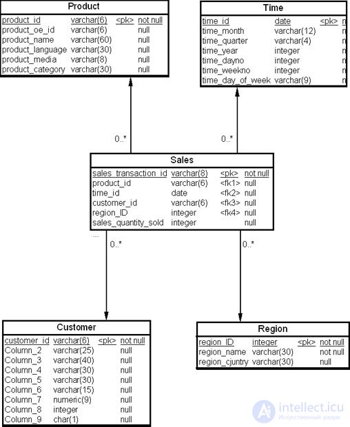
This data warehouse is designed for analyzing an organization's product sales system and includes, in addition to time, the following objects:
| Field name | Description |
|---|---|
| product_id | Product identifier |
| product_name | Product name |
| product_category | Product category |
| Field name | Description |
|---|---|
| time_id | Time identifier |
| time_month | Month |
| time_quarter | Quarter |
| time_year | Year |
| time_dayno | Day |
| time_weekno | Week |
| time_day_of_week | Day of week |
| Field name | Description |
|---|---|
| customer_id | Customer identifier |
| customer_name | Customer |
| customer_address | Address |
| customer_city | City |
| customer_subregion | District |
| customer_region | Region |
| customer_postalcode | Postal code |
| customer_age | Age |
| customer_gender | Customer type |
| Field name | Description |
|---|---|
| region_id | Region identifier |
| region_name | Region name |
| region_country | Country |
| Field name | Description |
|---|---|
| sales_transaction_id | Transaction identifier |
| product_id | Product identifier |
| customer_id | Customer identifier |
| time_id | Time identifier |
| region_id | Region identifier |
| sales_quantity_sold | Quantity of product sold |
| sales_dollar_amount | Dollar amount of product sold |
Thus, we end up with one fact table and four dimension tables. Let us consider how a SQL query against a "star" schema is constructed. A typical query against such a schema specifies detailed information about the points of this schema (i.e. the dimension), and then the data corresponding to those points is summarized.
Let us consider an example query against the schema shown in fig. 22.1.
Example 22.1. Suppose we need to view sales data for the product with identification number 33 for the months of May through August of the current year in the "Moscow" region with identification number 81. Then the query might look as follows:
SELECT SUM(sales_dollar_amount* sales_quantity_sold), time_month, region_name
FROM Sales, Time, Region
WHERE Sales.region_id = Region.region_id
   AND Sales.time_id = Time_time_id
   AND Sales.product_id = 33
   AND Sales.region_id = 81
   AND Time.time_month    BETWEEN 'Май' AND 'Август'
   AND Time.time_year = 2009
GROUP BY time_month, region_name
By changing the data for the region, months, and product, the above query can be used to reveal trends in sales data. The "star" schema is characterized by the use of one-way equi-joins between the dimension tables and the fact table. The dimension tables are not joined to each other.
The "Sales volume" metric examined in the previous example is an additive fact. Let us now consider how to construct queries for semi-additive facts.
The "Stock on hand" metric is a typical example of a semi-additive fact. Suppose that a store's warehouse calculates the balance for each product at the end of each month. Consider the "star" schema in fig. 22.2 for a data warehouse designed to analyze the movement of goods through a store.
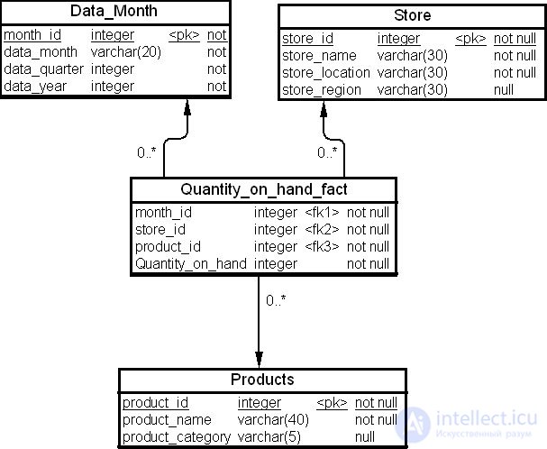
The schema presents three dimension tables: "Month" (Data_month), "Store" (Store), "Products" (Products), and the fact table "Stock on hand" (Quantity_on_hand_fact). The description of the tables is given in tab. 22.6 below.
| Field name | Description |
|---|---|
| "Month" dimension table (Data_month) | |
| month_id | Month identifier |
| data_month | Month |
| data_quarter | Quarter |
| data_year | Year |
| "Store" dimension table (Store) | |
| store_id | Store identifier |
| store_name | Store name |
| store_location | Store location |
| store_region | Region |
| "Products" dimension table (Products) | |
| product_id | Product identifier |
| product_name | Product name |
| product_category | Product category |
| "Stock on hand" fact table (Quantity_on_hand_fact) | |
| month_id | Month identifier |
| store_id | Store identifier |
| product_id | Product identifier |
| Quantity_on_hand | Stock on hand |
The "Stock on hand" metric is additive across the "Products" (Products) and "Store" (Store) dimensions, but is not additive across the "Month" (Data_month) dimension. Let us consider how the total quantity of products in stock at a store at any given point in time can be obtained, using the dimensions for which the semi-additive fact is additive.
Example 22.2. Suppose we need to sum the stock of the "Pillow" product across store warehouses for January 2009, taking into account the store locations, i.e. to determine how many unsold pillows were in the trading organization's chain of stores in January 2009. We do this by joining the fact table with the "Store" dimension, as shown below.
SELECT Store.store_location, SUM(Quantity_on_hand_fact.Quantity_on_hand)
FROM Store, Quantity_on_hand_fact, Products, Data_month
WHERE Store.store_id = Quantity_on_hand_fact.store_id
AND Quantity_on_hand_fact.month_id = Data_month.month_id
AND Products.product_id = Quantity_on_hand_fact.product_id
AND Data_month.data_month = 'Январь'
AND Data_month.data_year = 2009
AND Products.product_name ='Подушка'
GROUP BY Store.store_location
Similarly, the "Stock on hand" metric can be summed by the "Products" dimension to obtain the quantity of unsold products grouped by product category.
In the examples above, we used the aggregate function SUM() to sum values, and the GROUP BY clause to build the specified partitioning of the result set.
In a data warehouse, as a rule, a relation has an internal structure, and processing it requires partitioning the relation into subsets that share a particular value of a given attribute. For example, in a sufficiently general formulation the question can be stated as follows: tabulate the value of some function on each of these subsets according to the common value of the attribute.
The GROUP BY clause determines how to partition the original set into subsets according to a given criterion. The resulting partition represents the original relation as the union of a finite number of disjoint subsets. In particular, aggregate functions are applied sequentially to each subset individually, and the result of the function is output in the resulting relation.
Besides the SUM() function, the aggregate functions include: AVG() – computes the average value, MIN() – computes the minimum value, MAX() – computes the maximum value, COUNT() – computes the number of items in the result set (or in a partition element of the result set), and a number of others provided by the specific DBMS's SQL implementation.
The GROUP BY clause behaves like a projection with derived columns. It partitions the values in the specified columns into subsets according to the list of grouping columns. These subsets are characterized by identical values from the projection list. A projection onto these attributes is then performed, during which some derived column is computed and placed into an additional column of the resulting table.
There are restrictions on the use of grouping columns. Only columns from a given list — not any column from the table — may be specified as grouping columns in this SELECT clause. Specific SQL implementations provide for a whole additional range of restrictions.
Selection conditions can be applied to the results of executing the GROUP BY clause in order to exclude certain tuples from the resulting partition. The special HAVING clause is provided for this purpose, which specifies a selection condition on the attributes of the regrouped relation, rather than the original one. The main difference between the action of the HAVING clause's selection condition and the analogous selection condition of the WHERE clause is that the former selects entire subsets from the partition based on their aggregated properties, while the latter scans the contents of each of these subsets row by row, without taking the resulting partition into account. Sometimes the SELECT command executes faster using the HAVING clause than with the WHERE clause.
Vendors of industrial relational DBMSs strive to extend the analytical data processing capabilities of their SQL dialects. Such extensions to SQL capabilities are usually carried out in the following directions:
The CUBE and ROLLUP clauses make executing queries and building reports simpler in a data warehouse environment. The ROLLUP clause creates subtotals according to an increasing level of aggregation, from the most detailed levels of data representation to more generalized totals. The CUBE clause is an extension similar to the ROLLUP clause that allows all possible combinations of subtotals to be computed in a single command. The CUBE clause can generate the information needed for cross-tabulation reports (cross-tabulation reports) in a single query.
Analytic functions increase SQL's potential in the area of statistical processing of query result sets. Ranking functions include the computation of cumulative distributions, percent ranks, and partitioning into a given number of groups (N-tiles). Moving window computations enable working with cumulative aggregates (moving and cumulative aggregations), such as sums and averages.
Other SQL extensions include a family of functions for computing regressions, and CASE expressions. The regression computation functions include a full set of computations for linear regression. CASE expressions provide an implementation of if – then logic.
One of the key concepts of decision support systems (DSS) and executive information systems (EIS) is multidimensional analysis — the analysis of an object across all necessary combinations of dimensions. The term "dimension" is used to denote any category used to specify a query. The most common examples of dimensions in a data warehouse are "Time", "Geography", "Product", "Department", and "Distribution channel". Events or objects associated with specific dimension values are conventionally called facts. Examples of facts include "Sales", "Profit", "Number of customers", "Volume of production".
Typical examples of questions in multidimensional analysis are those which we will call multidimensional queries (MDQ).
All of the questions listed above use several dimensions. Many MDQs require aggregating data by time, geography, or finance, and comparing the resulting data sets.
To visualize data that has several dimensions, analysts use the analogy of a data cube, i.e. a portion of a multidimensional space in which facts are stored at the intersection of n dimensions. For example, a cube might store sales data organized along three dimensions — "Product", "Market", and "Time".
You can unfold (take slices of) data (slices of data) from the cube. This corresponds to the cross-tabular report shown in tab. 22.7. For example, a regional manager might study the data by comparing cube slices across different markets. A product manager might compare cube slices across different products.
Answering MDQs often requires accessing large amounts of data, aggregating that data across the levels of dimension hierarchies, and computing partial sums across dimensions. Thus, analytical tasks require efficient and convenient data aggregation.
Data aggregation capabilities are used not only in multidimensional analysis. Transaction processing, for example in financial or manufacturing systems (ERP), also generates a large number of reports. The efficiency of such systems increases when report generation does not overly constrain the load on the system. In the practice of financial and ERP systems, a large number of reports are generated at night, when the number of users of such systems drops significantly. It is important that database and data warehouse designers solve the problem of optimizing queries that use aggregation and summarization of data at various levels of detail, including such tasks as:
To illustrate SQL extensions in this lecture, we have taken a hypothetical data warehouse of an organization that sells and rents out video cassettes. The data warehouse stores information about the organization's operations in several regions, tracking sales and profit from sales. Data is stored along three dimensions – "Time" (Time), "Sales department" (Department), and "Region" (Region). The time period of the data spans from 2000 to 2009. The company has two types of sales departments – the "Retail sales department" (Video Sales) and the "Video rental department" (Video Rentals). The region includes three areas: "Central" (Central), "East" (East), and "West" (West). The "Sales" fact table (Sales) contains data on the company's sales and rentals of video products for 2000-2009. The "star" schema for this data warehouse is shown in fig. 22.3, and the description of the dimension table and fact table fields is given in tab. 22.7.
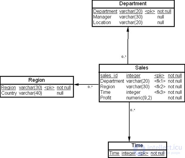
| Field name | Description |
|---|---|
| "Time" dimension table (Time) | |
| Time | Year |
| "Region" dimension table (Region) | |
| Region | Region name |
| Country | Country |
| "Sales departments" dimension table (Department) | |
| Department | Sales department |
| Manager | Department head |
| Location | Location |
| "Sales" fact table (Sales) | |
| sales_id | Sale identifier |
| Time | Year |
| Region | Region name |
| Department | Sales department |
| Profit | Profit |
Tab. 22.8 shows a typical report that company management might request to analyze the company's performance over a given period of time.
| 2008 | |||
|---|---|---|---|
| Region | Sales department | ||
| Rental profit | Sales profit | Total profit | |
| Central | 82,000 | 85,000 | 167,000 |
| East | 101,000 | 137,000 | 238,000 |
| West | 96,000 | 97,000 | 193,000 |
| Total | 279,000 | 319,000 | 598,000 |
Note that this small report generates five subtotals plus the grand totals. The subtotals are hidden numbers that must be computed for the report in a query using the aggregate function SUM() and the GROUP BY clause.
Let us now examine in more detail the extensions to the SELECT statement that simplify the construction of queries for building reports similar to the one shown in tab. 22.7.
The ROLLUP clause allows a SELECT command to compute multi-level subtotals for specified groups of dimensions. It also computes a grand total. The ROLLUP clause is a simple extension of the GROUP BY clause, so its syntax is straightforward to use. Using the ROLLUP clause is very efficient.
Syntax:
SELECT ... GROUP BY ROLLUP(grouping_column_reference_list)
The actions of ROLLUP are as follows: subtotals are created for each of the levels being expanded, from the lowest level of the hierarchy to a higher level, and a grand total is computed according to the specified list of columns in the ROLLUP clause. The ROLLUP clause treats its arguments as an ordered list of grouping columns. First, the standard aggregate value specified in the GROUP BY clause is computed. Then subtotals are created for the levels of attributes from the GROUP BY grouping list in increasing order of their values, from right to left across the list of grouping columns. And finally the grand total is created.
The ROLLUP clause creates subtotals for n+1 levels, where n is the number of grouping columns. For example, if a query specifies ROLLUP on the grouping columns of the "Time" (Time), "Region" (Region), and "Sales department" (Department) dimensions ( n=3 ), then the result set (result set) will include rows for 4 levels of aggregation.
Let us consider examples.
Example 22.3. Suppose company management requires a profit report across all regions and all sales departments for 2007-08. The SELECT clause for the data warehouse schema shown in fig. 22.3 might look as follows.
SELECT Time, Region, Department, SUM(Profit) AS Profit
FROM sales
   GROUP BY ROLLUP(Time, Region, Department);
Output 1: ROLLUP aggregation for three dimensions
| Time | Region | Department | Profit |
|---|---|---|---|
| 2007 | Central | VideoRental | 75,00 |
| 2007 | Central | VideoSales | 74,00 |
| 2007 | Central | NULL | 149,00 |
| 2007 | East | VideoRental | 89,00 |
| 2007 | East | VideoSales | 115,00 |
| 2007 | East | NULL | 204,00 |
| 2007 | West | VideoRental | 87,00 |
| 2007 | West | VideoSales | 86,00 |
| 2007 | West | NULL | 173,00 |
| 2007 | NULL | NULL | 526,00 |
| 2008 | Central | VideoRental | 82,00 |
| 2008 | Central | VideoSales | 85,00 |
| 2008 | Central | NULL | 167,00 |
| 2008 | East | VideoRental | 101,00 |
| 2008 | East | VideoSales | 137,00 |
| 2008 | East | NULL | 238,00 |
| 2008 | West | VideoRental | 96,00 |
| 2008 | West | VideoSales | 97,00 |
| 2008 | West | NULL | 193,00 |
| 2008 | NULL | NULL | 598,00 |
| NULL | NULL | NULL | 1124,00 |
As can be seen from the example above, the query returns the following set of rows:
Note that the NULL values are shown here only for clarity. In actual output, blank spaces would be displayed instead.
The NULL values returned as a result of the ROLLUP and CUBE clauses cannot always be interpreted in the usual sense, as undefined values. A NULL value may indicate that the row contains a partial sum. For example, the first NULL value in Output 1 appears in the "Department" column. This NULL value means that the row is a partial sum across all sales departments for the Central region in 2007.
The ROLLUP clause can be used to compute only some partial sums. Such commands using ROLLUP use the syntax shown below:
GROUP BY expr1, ROLLUP(expr2, expr3);
In this case, the ROLLUP clause creates partial sums for (2+1=3) aggregation levels, i.e., for the levels (expr1, expr2, expr3), (expr1, expr2), and (expr1). The grand total is not created.
Example 22.4. Suppose company management requires a profit report across all regions and all sales departments for 2007-2008, without the profit grand total. The SELECT statement for the data warehouse schema shown in Fig. 22.3 might look as follows:
SELECT Time, Region, Department, SUM(Profit) AS Profit FROM sales
   GROUP BY Time, ROLLUP (Region, Department);
Output 2. Using the ROLLUP clause to output partial sums
| Time | Region | Department | Profit |
|---|---|---|---|
| 2007 | Central | VideoRental | 75,00 |
| 2007 | Central | VideoSales | 74,00 |
| 2007 | Central | NULL | 149,00 |
| 2007 | East | VideoRental | 89,00 |
| 2007 | East | VideoSales | 115,00 |
| 2007 | East | NULL | 204,00 |
| 2007 | West | VideoRental | 87,00 |
| 2007 | West | VideoSales | 86,00 |
| 2007 | West | NULL | 173,00 |
| 2007 | NULL | NULL | 526,00 |
| 2008 | Central | VideoRental | 82,00 |
| 2008 | Central | VideoSales | 85,00 |
| 2008 | Central | NULL | 167,00 |
| 2008 | East | VideoRental | 101,00 |
| 2008 | East | VideoSales | 137,00 |
| 2008 | East | NULL | 238,00 |
| 2008 | West | VideoRental | 96,00 |
| 2008 | West | VideoSales | 97,00 |
| 2008 | West | NULL | 193,00 |
| 2008 | NULL | NULL | 598,00 |
As can be seen, the query returns the following set of rows:
Partial sums can be computed without using the ROLLUP clause as follows:
SELECT Time, Region, Department, SUM(Profit)
 FROM Sales
 GROUP BY Time, Region, Department
UNION  ALL
 SELECT Time, Region, '' , SUM(Profit)
 FROM Sales
 GROUP BY Time, Region
UNION ALL
 SELECT Time, '', '', SUM(Profit)
 FROM Sales
 GROUP BY Time
UNION ALL
 SELECT '', '', '', SUM(Profit)
 FROM Sales;
As can be seen from the example above, this requires n+1 SELECT statements with UNION ALL for n dimensions.
It makes sense to use the ROLLUP clause for tasks that compute intermediate or partial sums:
The partial sums generated by the ROLLUP clause represent only part of the possible combinations of partial sums across dimensions. For example, in a cross-tab report (see Table 22.1), the department totals by region (279,000 and 319,000) cannot be computed by the clause ROLLUP(Time, Region, Department). To achieve this, the column grouping order in the ROLLUP clause would need to be changed: ROLLUP(Time, Department, Region). A simple way to generate the full set of partial sums for cross-tab reports is to use the CUBE extension of the GROUP BY clause.
The CUBE clause allows a SELECT statement to compute partial sums for all possible combinations of the grouped dimensions. It also computes the grand total. Like ROLLUP, the CUBE clause is an extension of the GROUP BY clause.
Syntax:
SELECT ...  GROUP BY
  CUBE (grouping_column_reference_list)
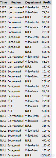
From the example below it can be seen that CUBE takes the specified set of grouping columns and creates partial sums for all possible combinations of the values in these columns. From the perspective of multidimensional analysis, the CUBE clause generates all partial sums that can be computed for a data cube with the specified dimensions. If CUBE(Time, Region, Department) is specified, the query result set will include all the values included in the equivalent ROLLUP construct, plus a set of additional combinations.
Example 22.5. Suppose company management requires a cross-tab profit report across all regions and all sales departments for 2007-2008. The SELECT statement for the data warehouse schema shown in Fig. 22.3 might look as follows:
SELECT Time, Region, Department, SUM(Profit) AS Profit
FROM sales
   GROUP BY CUBE(Time, Region, Department);
Output 3. Executing CUBE with aggregation across three dimensions
Using CUBE to compute partial sums is similar to using the ROLLUP clause to compute partial sums, in that the use of some dimensions can be restricted. In this case, the computation of all possible combinations is limited to the dimensions specified in the grouping list.
Syntax:
GROUP BY expr1, CUBE(expr2, expr3);
As a result of executing this command, 4 partial sums will be computed:
Example 22.6. Suppose company management requires a cross-tab profit report across all regions and all sales departments for 2007-2008, without output of partial sums. The SELECT statement for the data warehouse schema shown in Fig. 22.3 might look as follows:
SELECT Time, Region, Department, SUM(Profit) AS Profit FROM sales
   GROUP BY Time CUBE(Region, Department);
Output 4. Using CUBE to compute partial sums
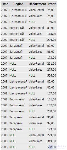
Without using the CUBE clause, an n-dimensional cube would require 2n SELECT statements with UNION ALL.
It makes sense to use the CUBE clause when solving tasks that involve building cross-tab reports.
The DISTINCT qualifier has erroneous semantics within ROLLUP and CUBE clauses. It is not recommended to use the DISTINCT qualifier in combination with these clauses.
Two problems arise when using ROLLUP and CUBE. The first: how can one programmatically determine which rows of the result set are partial sums, and how does one find the exact aggregation level of a given partial sum? Partial sums are often needed for computing percentage ratios between totals, so a simple way to find partial sums is needed. The second problem: what happens if the query result contains both NULL values from stored rows and pseudo-NULL values created by ROLLUP or CUBE? How can they be distinguished in the result set?
The GROUPING function is designed to solve this problem. It is a statistical function that produces an additional column containing the value 1 if the row was added by the CUBE or ROLLUP operator, or the value 0 otherwise.
Syntax (specified in the list of the SELECT clause):
SELECT ...  [GROUPING(column_name)...]  ...
  GROUP BY ...    {CUBE | ROLLUP}  (column_name)
Example 22.7. Using the GROUPING function to create mask columns in the result set.
SELECT Time, Region, Department, SUM(Profit) AS Profit,
  GROUPING (Time) as T,
  GROUPING (Region) as R,
  GROUPING (Department) as D
  FROM Sales
GROUP BY ROLLUP (Time, Region, Department);
Output 5. Using the GROUPING function
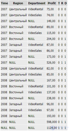
As can be seen from the example, the mask "0 0 0" is a row aggregated from the table, "0 0 1" is the first aggregation level, "0 1 1" is the second aggregation level, and "1 1 1" is the grand total.
Example 22.8. Suppose a SELECT statement produces the following result set, created by the CUBE expression.
Output 6.
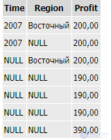
The result set contains 4 different rows with NULL values in the "Time" and "Region" columns. Some of these NULL values must represent CUBE aggregates, while others represent NULL values stored in the database. How can the aggregate NULL values built by the CUBE clause be distinguished in the report from the NULL values stored in the database?
Using the GROUPING function in combination with a CASE expression and the data type conversion function CAST (expression AS data_type [ (length ) ]) makes it possible to solve this problem.
The CASE expression evaluates a list of conditions and returns one of several possible result expressions.
Syntax:
CASE input_expression
     WHEN when_expression THEN result_expression [ ...n ]
     [ ELSE else_result_expression ]
END
or
CASE
     WHEN Boolean_expression THEN result_expression [ ...n ]
     [ ELSE else_result_expression ]
END
Now the report from Example 22.8 can be transformed so as to highlight the CUBE clause's aggregates, as shown below.
Example 22.9. Distinguishing aggregate NULL values from stored NULL values.
SELECT
CASE WHEN GROUPING(Time) = 1 THEN 'All Times' ELSE CAST(Time as CHAR(20)) END AS Time,
CASE WHEN GROUPING(Region) = 1 THEN 'All Regions' ELSE Region END AS Region, SUM(Profit) AS Profit
FROM Sales
GROUP BY CUBE(Time, Region);
Output 7. Distinguishing aggregate NULL values from stored NULL values
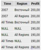
The first column is "Time," defined by the expression
CASE WHEN GROUPING(Time) = 1 THEN 'All Times' ELSE CAST(Time as CHAR(20)) END AS Time,
The value of Time is defined by a CASE expression containing the GROUPING function. The GROUPING function returns 1 if the row is an aggregate produced by the ROLLUP or CUBE clause, and 0 otherwise. CASE operates on the result of the GROUPING function. It returns the text "All Times" if that result is 1, and the value of the "time" column from the database if it is 0. Database values will be either an actual value, such as 2007, or a stored NULL value. The CAST function is used to reconcile types, since all columns in the result set must be of the same type. The second column in the specification, showing the values of the "Region" column, is handled in a similar way.
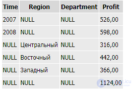
The GROUPING function is useful not only for identifying NULL values — it can also help sort partial sum rows and filter the result set. In the example below, a subset of the partial sums created by CUBE is selected. The HAVING clause restricts the columns used in the GROUPING function.
Example 22.10.
SELECT Time, Region, Department, SUM(Profit) AS Profit,
  GROUPING (Time) AS T,
  GROUPING (Region) AS R,
  GROUPING (Department) AS D
  FROM Sales
  GROUP BY CUBE (Time, Region, Department)
  HAVING (GROUPING(Department)=1 AND GROUPING(Region)=1 AND GROUPING(Time)=1)
  OR (GROUPING(Region)=1 AND (GROUPING(Department)=1)
  OR (GROUPING(Time)=1 AND GROUPING(department)=1);
Output 8. Example of using the GROUPING function to filter the result set to partial sums and the grand total
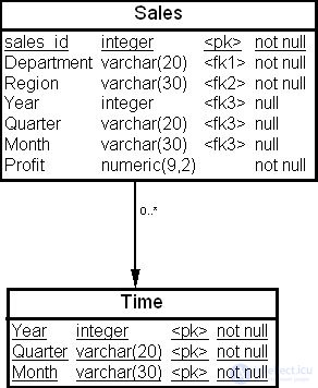
The ROLLUP and CUBE clauses work independently of any hierarchy present in the data in the database. Their computations are based on the columns that appear in the list of the SELECT statement. This approach makes it possible to use CUBE and ROLLUP for processing hierarchies as well. A simple way to manage a dimension's hierarchy is to use the ROLLUP clause and precisely specify the hierarchy levels for the selected column. The example below shows how months are rolled up into quarters, and quarters into years. This assumes that the training example's data warehouse schema has been modified as shown in Fig. 22.4.
Example 22.11.
SELECT Year, Quarter, Month, SUM(Profit) AS Profit
FROM sales
   GROUP BY ROLLUP(Year, Quarter, Month)
HAVING Year = 2008;
Output 9. Example of ROLLUP using the hierarchy levels of the "Time" dimension
| Year | Quarter | Month | Profit |
|---|---|---|---|
| 2008 | First | January | 55,00 |
| 2008 | First | February | 64,00 |
| 2008 | First | March | 71,00 |
| 2008 | First | NULL | 190,00 |
| 2008 | Second | April | 75,00 |
| 2008 | Second | May | 86,00 |
| 2008 | Second | June | 88,00 |
| 2008 | Second | NULL | 249,00 |
| 2008 | Third | July | 91,00 |
| 2008 | Third | August | 87,00 |
| 2008 | Third | September | 101,00 |
| 2008 | Third | NULL | 279,00 |
| 2008 | Fourth | October | 109,00 |
| 2008 | Fourth | November | 114,00 |
| 2008 | Fourth | December | 133,00 |
| 2008 | Fourth | NULL | 356,00 |
| 2008 | NULL | NULL | 1074,00 |
Let us note a few features of using the ROLLUP and CUBE clauses.
The CUBE and ROLLUP clauses do not limit the column capacity of the GROUP BY clause. The GROUP BY clause, with or without extensions, can work with up to 255 columns. However, the number of combinations that the CUBE clause creates can be very large. For 20 columns, the CUBE clause would create 220 combinations in the result set.
The HAVING clause of the SELECT statement does not affect the use of the ROLLUP and CUBE clauses in the sense that it applies to the GROUP BY clause as a whole. The predicate in the HAVING clause applies both to partial-sum rows and to aggregate rows of the result set.
The ORDER BY clause of the SELECT statement does not affect the use of the ROLLUP and CUBE clauses. The predicate in the ORDER BY clause applies to all rows of the result set.
In this lecture, we examined the extensions of the SELECT statement's GROUP BY clause intended for aggregating data in the result set.
Using the CUBE and ROLLUP clauses makes running queries and building reports simpler in a data warehouse environment. The ROLLUP clause is best suited to tasks that compute intermediate or partial sums, while the CUBE clause is best suited to solving tasks that involve building cross-tab reports.
In conclusion, let us give the detailed syntax of the GROUP BY clause in the SQL dialect of the MS SQL Server DBMS family.
Syntax compliant with the ISO/IEC 9075-5 standard:
GROUP BY <group by spec>

<group by spec> ::=
    <group by item> [ ,...n ]

<group by item> ::=
    <simple group by item>
    | <rollup spec>
    | <cube spec>
    | <grouping sets spec>
    | <grand total>

<simple group by item> ::=
    <column_expression>

<rollup spec> ::=
    ROLLUP ( <composite element list> )

<cube spec> ::=
    CUBE ( <composite element list> )

<composite element list> ::=
    <composite element> [ ,...n ]

<composite element> ::=
    <simple group by item>
    | ( <simple group by item list> )

<simple group by item list> ::=
    <simple group by item> [ ,...n ]

<grouping sets spec> ::=
    GROUPING SETS ( <grouping set list> )

<grouping set list> ::=
    <grouping set> [ ,...n ]

<grouping set> ::=
    <grand total>
    | <grouping set item>
    | ( <grouping set item list> )

<empty group> ::=
        ( )

<grouping set item> ::=
    <simple group by item>
    | <rollup spec>
    | <cube spec>

<grouping set item list> ::=
    <grouping set item> [ ,...n ]
Listing .Syntax not covered by the ISO/IEC 9075-5 standard:
[ GROUP BY [ ALL ] group_by_expression [ ,...n ]
    [ WITH { CUBE | ROLLUP } ]
]
<column_expression>

Comments