Analytical data processing in data warehouses (analytic, statistical, ranking, window, and reporting functions)

SQL for Data Analysis

In this lecture we will focus on the capabilities that SQL provides for the analytical processing of data in a data warehouse. In the examples given, we will follow the Transact-SQL dialect of the MS SQL Server family of DBMSs.

Note that, on the whole, SQL does not have good support for solving analytical problems. However, the built-in support for analytic functions in Transact-SQL, and its set-oriented nature, make it a good tool for performing such computations over data stored in a data warehouse. Analytic functions and the set-oriented approach give Transact-SQL certain advantages over other data manipulation languages.

The main computations in business intelligence systems — computing a moving average, ranking a sample, and so on — require a large amount of programming in standard SQL. Functions of this type are called analytic functions.

Analytic functions fall into the following categories:

• statistical functions;
• ranking functions;
• window functions;
• reporting functions.

Table 23.1 gives a brief description of the categories of analytic functions.

To perform these operations, several elements have been added to SQL command processing. These elements are built into SQL. There are several new concepts used by analytic functions.

• Processing Order. Queries that use analytic functions are processed in three stages. The first includes all joins, WHERE, GROUP BY, and HAVING. The second is the application of the analytic functions to the result set. The third — if there is an ORDER BY clause, it is processed.
• Result Set Partitions. Analytic functions let the user divide the query's result set into groups of rows called partitions. The term "partition" is used here in a different sense from the one used for table partitioning. Here it denotes the groups created after grouping by the GROUP BY clause. These partitions are built according to the value of the grouping column.
• Window. For each row in a partition you can define a sliding window of data. This window defines the range of rows used for computations relative to the current row. The window size can be specified either as a physical number of rows or as a logical number of rows (a condition). A window has a starting row and an ending row. Depending on its definition, the window can move across the result set at one or both ends. For example, a window defined for a cumulative sum function will have the first row of the partition as its starting row, and its ending row will slide from the starting point all the way to the last row of the partition. In contrast, a window defined for a moving average will have both its starting and ending points sliding so as to capture a constant physical or logical interval.
• Current Row. Every computation with analytic functions is based on the current row within a partition. The current row is maintained as a reference to a row (position) inside the window. For example, computing a centered moving average may require defining a window with 5 rows preceding the current row and 6 rows following it. The window will be 12 rows in size.

Aggregate and Statistical Functions

Transact-SQL supports nine different aggregate functions needed for statistical computations. In addition to the aggregate functions already mentioned in the previous lecture — SUM(), MIN(), MAX(), COUNT(), and AVG() — there are four more intended specifically for financial and statistical calculations: STDEV(), STDEVP(), VAR(), VARP() (Table 23.2).

Statistical functions perform a computation on a set of values and return a single value. Except for the COUNT function, these functions ignore NULL values. They are also often used with the GROUP BY clause of the SELECT statement.

These functions can be used as expressions only in the following cases:

• the select list of a SELECT statement (a nested or outer query);
• a COMPUTE or COMPUTE BY clause;
• a HAVING clause.

AVG ( [ ALL | DISTINCT ] expression )

CHECKSUM_AGG ( [ ALL | DISTINCT ] expression )

COUNT ( { [ [ ALL | DISTINCT ] expression ] | * } )

COUNT_BIG ( { [ ALL | DISTINCT ] expression } | * )

GROUPING ( <column_expression> )

MAX ( [ ALL | DISTINCT ] expression )

MIN ( [ ALL | DISTINCT ] expression )

SUM ( [ ALL | DISTINCT ] expression )

STDEV ( [ ALL | DISTINCT ] expression )

STDEVP ( [ ALL | DISTINCT ] expression )

VAR ( [ ALL | DISTINCT ] expression )

VARP ( [ ALL | DISTINCT ] expression )

The ALL keyword applies the function to all values. ALL is the default argument, while DISTINCT indicates that each unique value is considered.

Let us look at an example in which built-in aggregate functions are used to compute basic statistical parameters.

Example 23.1. Aggregate and statistical functions

Suppose the data warehouse contains a fact table "Population" ( Population ), whose contents are shown in Table 23.3, and a dimension table "Region" ( Region ), whose physical structure is shown in Fig. 23.1.

Fig. 23.1. Physical structure of the fact table "Population" (Population) and the dimension table "Region" (Region)

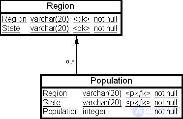
The SELECT statement below illustrates the use of aggregate and statistical functions.

SELECT Region. MIN(Population) AS Minimum, MAX(Populations)AS Maximum,
AVG(Population) AS Average. VAR(Population) AS Variance
FROM Region
GROUP BY Region
ORDER BY Maximum DESC

The result of executing the query is shown below.

Output 1.

Example 23.2. Using GROUPING

Suppose we need to perform statistical processing of the values in the "Sale Volume" (Sale) column, grouped by the "Quota" (Quota) column in the "Sales" (Sales) table, whose structure is shown in Fig. 23.2. The GROUPING function is applied to the Quota column.

Fig. 23.2. Physical structure of the "Sales" (Sales) table

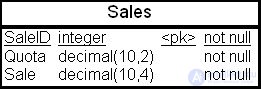
The following query solves the stated problem:

SELECT Quota, SUM(Sale) 'TotalSales', GROUPING(Quota) AS 'Grouping'
FROM Sales
GROUP BY Quota WITH ROLLUP;
GO

The result set shows two NULL values in the Quota column. The first NULL value represents the group of NULL values from that column in the table. The second NULL value is in the summary row added by the ROLLUP operation. The summary row shows the sums of TotalSales for all Quota groups and is denoted by a 1 in the Grouping column.

The result of executing the query is shown below.

Output 2.

Many statistical functions are used in applied statistics. In the next section we will show how to compute some of them using SQL.

Medians

The task of positioning records, or finding records based on their physical location within a sample, has historically been difficult to solve using SQL. Finding a record by value is quite simple in set-oriented languages; finding a record by position, however, is a difficult task.

The task of finding medians is a record-positioning task. If the sample has an odd number of records, the median value equals the value of the record located exactly in the middle of the sample. There is an equal number of elements above and below this value. If the sample has an even number of values, the median value equals either the average of the two central values (in the case of financial medians), or the smaller of the two (in the case of statistical medians).

The task of positioning records becomes considerably simpler when the table has a unique sequential integer key (an identity column). If so, the key becomes a virtual record number, and it becomes possible to access records at any position of the table as if it were an array. Because of this, we can compute medians almost instantly even for samples consisting of millions of values.

Example. 16.3. Computing the median.

Suppose the data warehouse contains a fact table "Finance" (Finance) containing several million values of product prices. The physical structure of the table is shown in Fig. 23.3. The ID column was created with the identity type qualifier. The records are sorted by the value of the "Price" (Price) column by creating a clustered index, for which the ID column was added — that is, the records were simply renumbered. The index on the "Price" (Price) column was dropped, and one was created on the ID column instead.

Fig. 23.3. Physical structure of the fact table "Finance" (Finance)

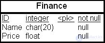
The following query computes the financial median:

SELECT AVG(Price) AS "Финансовая медиана" FROM finance
WHERE ID BETWEEN MAX(ID) / 2 AND (MAX(ID) / 2) + SIGN(MAX{(ID) +1 % 2)

The SIGN() function is used to handle both even and odd numbers of records within a single BETWEEN clause. The expression with this function adds 1 to the number of records in the sample to flip it from even to odd or vice versa, then computes the remainder of division by 2 to determine whether the number is even or odd, and returns 1 or 0 depending on the sign.

Window Functions

Window functions are defined in the ISO SQL standard. DBMSs of the MS SQL Server family provide ranking and statistical window functions. A window is a user-defined set of rows. A window function computes a value for each row in the result set derived from the window.

Window functions can be used to compute cumulative, moving, and centered aggregates. They return a value for each row in the table that depends on other rows of the corresponding window. They can only be used in the SELECT and ORDER BY clauses of a query. As a rule, window functions provide access to more than one row of the table without a self-join.

The OVER Clause

The OVER clause defines the partitioning and ordering of a row set before the corresponding window function is applied. Aggregate and statistical functions ( SUM, AVG, MAX, MIN, COUNT ) and ranking functions are used as window functions. Each of the ranking functions ROW_NUMBER, DENSE_RANK, RANK, and NTILE makes use of the OVER clause (see the next section of this lecture).

Syntax:

• For ranking window functions

  < OVER_CLAUSE > ::= OVER ( [PARTITION BY value_expression, … [n] ] <ORDER BY expression>)
• For aggregate functions

  < OVER_CLAUSE > ::= OVER ( [PARTITION BY value_expression, … [n] ]

PARTITION BY divides the result set into partitions. The window function is applied to each partition separately, and the computation starts over for each partition. If this clause is omitted, the function treats the entire result set as a single group.

value_expression specifies the column by which the row set produced by the corresponding FROM clause is partitioned. The value_expression argument can only reference columns available through the FROM clause. The value_expression argument cannot reference expressions or aliases in the select list. The value_expression can be a column expression, a scalar subquery, a scalar function, or a user variable.

The ORDER BY clause specifies the order for a ranking window function. If the ORDER BY clause is used in the context of a ranking window function, it can only reference columns available through the FROM clause. You cannot specify the position of a column name or alias in the select list by an integer. The ORDER BY clause cannot be used with statistical window functions.

A single query with a single FROM clause can use several statistical or ranking window functions. However, the OVER clause for each function can apply its own partitioning and ordering. The OVER clause cannot be used with the statistical function CHECKSUM.

The NULL-value semantics of window functions matches the NULL-value semantics of SQL aggregate functions.

Statistical Window Functions

Let us show, using an example, how statistical window functions are used.

Example. 16.4. Statistical window functions.

Suppose the data warehouse contains a fact table "Order Line Items" (OrderDetail) containing the line number (OrderID), product identifier (ProductID), product quantity (OrderQty), and product price (Price). The physical structure of the table is shown in Fig. 23.4.

Fig. 23.4. Physical structure of the fact table "Finance" (Finance)

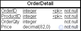
Suppose that for two order lines, 43659 and 43664, we need to compute, for each product sold, the total quantity sold, the average quantity of each product sold, and the minimum and maximum quantity sold.

The following query solves the stated problem using window functions.

SELECT OrderID, ProductID, OrderQty
	,SUM(OrderQty) OVER(PARTITION BY OrderID) AS 'Итого'
	,AVG(OrderQty) OVER(PARTITION BY OrderID) AS 'Среднее'
	,COUNT(OrderQty) OVER(PARTITION BY OrderID) AS 'Кол-во'
	,MIN(OrderQty) OVER(PARTITION BY OrderID) AS 'Min'
	,MAX(OrderQty) OVER(PARTITION BY OrderID) AS 'Max'
FROM OrderDetail
WHERE OrderID IN(43659,43664);
GO

The result of executing the query is shown below.

Output 3.

Suppose the management of the organization requires calculating the percentage of product sold for order line 43659. The following query using window functions solves the stated problem.

SELECT OrderID, ProductID, OrderQty
	,SUM(OrderQty) OVER(PARTITION BY OrderID) AS 'Итого'
	,CAST(1. * OrderQty / SUM(OrderQty) OVER(PARTITION BY 	OrderID) *100 AS DECIMAL(5,2))AS 'Процент проданного товара'
FROM OrderDetail
WHERE OrderID = 43659;

The result of executing the query is shown below.

Output 4.

As the examples above show, using the OVER clause is more efficient than using nested queries. The application of window ranking functions will be covered in the next section.

Ranking functions

Ranking functions compute the rank of a row relative to the other rows in a dataset, based on the value of a set of measures. They return a ranking value for each row in a partition. Depending on the function used, some rows may end up with the same value.

The types of ranking functions are shown in Table 23.4.

The RANK and DENSE_RANK functions

The RANK and DENSE_RANK functions let you rank items within a group — for example, to find the top 3 products sold in California over the last year. There are two ranking functions with the following syntax:

RANK ( ) OVER ( [ < partition_by_clause > ] < order_by_clause > )

< partition_by_clause > ([PARTITION BY <value expression1> [, ...]]) divides the result set produced by the FROM clause into partitions to which the RANK function is applied.

< order_by_clause > ( ORDER BY <value expression2> [collate clause] [ASC|DESC] ) determines the order in which the RANK values are applied to the rows in the partition. An integer value cannot represent a column in the < order_by_clause > when used in a ranking function.

If two or more rows tie for the same rank, they will all receive the same rank. For example, if the top two salespeople have the same sales volume, they will both be assigned rank 1. The sales manager with the next-highest sales volume will get rank number 3, since there are two rows with a higher rank ahead of them. That is why the RANK function does not always return consecutive integers.

The sort order used for the query as a whole determines the order in which rows appear in the result set.

DENSE_RANK ( ) OVER ( [ < partition_by_clause > ] < order_by_clause > )

< partition_by_clause > divides the result set produced by the FROM clause into partitions to which the DENSE_RANK function is applied.

< order_by_clause > determines the order in which DENSE_RANK values are applied to the rows of a partition. An integer cannot represent a column in the <order_by_clause> used in a ranking function.

If two or more rows within a partition tie in the ranking, each such row is assigned the same rank. For example, if the top two salespeople have the same sales volume, they will both be assigned rank 1. The salesperson with the next-highest sales volume is assigned rank 2 — one more than the number of distinct ranks of the rows preceding that row. Thus there are no gaps between the numbers returned by the DENSE_RANK function, and they always form a sequence of consecutive rank values.

The sort order of rows in the result is determined by the sort order of the entire query's result. It follows that a row with rank 1 is not always the first row in the partition.

Thus, the difference between RANK and DENSE_RANK is that DENSE_RANK leaves no gaps in the ranking sequence.

It is recommended to use the RANK function when:

• the default sort order for these functions is ascending order;
• the expressions in the PARTITION BY clause divide the result set of the query into groups over which the RANK function operates, and the function resets when moving to the next group. In effect, the <value expression> of the PARTITION BY clause defines the scope of the function;
• the PARTITION BY clause is omitted, in which case the rank is computed over the entire result set of the query;
• the ORDER BY clause defines the metrics ( <value expressions> ) on which the rank is computed, and defines the order in which rows are sorted within each group or partition. Once the data is sorted within each partition, ranks are assigned to each row starting from 1;
• <value expression2> can be any valid expression, including references to columns, aggregates, or expressions built from these elements.

Let's look at a number of examples of applying ranking functions.

Ranking can be performed on multiple expressions. Ranking functions are needed to find a relationship among values across a set of records. If the first expression cannot resolve the relationship, the second is used to resolve it, and so on.

Example 23.5. Using the RANK() function.

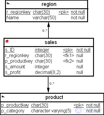
Suppose we need to rank products based on sales in rubles in each region, breaking ties using revenue. The physical schema of the data mart is shown in Fig. 23.5.

The schema shows the "Sales" fact table (sale) with the measures "Quantity" (s_amount) and "Profit" (s_profit), and two dimension tables, "Region" (region) and "Product" (product).

The following query solves the stated problem:

SELECT r_regionkey, p_productkey, s_amount, s_profit,
  RANK() OVER (ORDER BY s_amount DESC, s_profit DESC) AS 'Ранг по востоку'
FROM region, product, sales
WHERE region.r_regionkey = sales.s_regionkey AND product.p_productkey = sales.s_productkey AND r_regionkey = 'Восток';

Fig. 23.5. Physical schema of the data mart

The query result is shown below.

Output 5.

For jackets and trousers, the "Revenue" column (s_profit) shows a correlation with the "Quantity" column (s_amount). But for sweaters and shirts, the "Revenue" column cannot establish a correlation with the "Quantity" column. Consequently, they are assigned the same rank.

The difference between RANK() and DENSE_RANK() can be illustrated with a query against the "Sales" fact table:

SELECT р_productkey, SUM(s_amount) as 'Суммарное количество',
  RANK() OVER (ORDER BY SUM(s_amount) DESC) AS 'rank_all',
  DENSE_RANK() OVER (ORDER BY SUM(s_amount) DESC) AS 'rank_dense'
FROM sales
GROUP BY р_productkey;

The query result is shown below.

Output 6.

As can be seen in the result set, in the case of the DENSE_RANK() function, the highest rank value equals the number of distinct values in the dataset.

The RANK() function can be applied for operations within groups, i.e., the rank resets when the data group changes. This is important for the PARTITION BY option. The grouping expression in PARTITION BY singles out subclasses of data within the dataset on which RANK operates.

Example 23.6. We need to rank products in each region by their sales in rubles. We can write a query against the schema in Fig. 23.5 that ranks products based on their sales in rubles within each region ( rank_of_product_per_region ) and across all regions ( rank_of_product_total ).

SELECT r_regionkey, p_productkey, SUM(s_amount) AS 'SUM_S_AMOUNT',
RANK() OVER (PARTITION BY r_regionkey ORDER BY SUM(s_amount) DESC)
AS 'rank_of_product_per_region',
RANK() OVER (ORDER BY SUM(s_amount) DESC) AS 'rank_of_product_total'
FROM product, region, sales
WHERE region.r_regionkey = sales.r_regionkey AND product.p_productkey = sales.p_productkey
GROUP BY r_regionkey, p_productkey
ORDER BY r_regionkey;

The query result is shown below.

Output 7.

The NTILE function

The NTILE() function divides an ordered partition into a specified number of groups called buckets ( buckets ), and assigns a bucket number to each row in the partition. For each row, the NTILE() function returns the number of the group to which the row belongs. NTILE() — is a very useful function since it lets you split a dataset into 40, 30, or any other number of groups.

Buckets are computed so that each one gets either the same number of rows, or one more. For example, if there are 100 rows in a partition and the NTILE function is applied for 4 buckets, then 25 rows will be assigned to each bucket.

If the number of rows in a partition does not divide evenly (by the number of buckets), the number of rows initially assigned to each bucket will differ by at least 1. For example, if there are 103 rows in a partition to which the NTILE(5) function is applied, the first 21 rows will be assigned to bucket 1, the next 21 to bucket 2, the next 21 to bucket 3, the next 20 to bucket 4, and the last 20 to bucket 5.

Syntax:

NTILE (integer_expression)    OVER ( [ <partition_by_clause> ] < order_by_clause > )

integer_expression - a positive integer constant expression specifying the number of groups into which each partition must be divided. The integer_expression argument can be of type int or bigint.

<partition_by_clause> divides the result set formed by the FROM clause.

< order_by_clause > determines the order in which the values of the NTILE function are assigned to the rows of the partition.

The integer_expression argument can only reference columns in the PARTITION BY clause and cannot reference columns listed in the current FROM clause.

Example 23.7. Using the NTILE() function

Suppose we need to group the products sold by sales volume, using the schema in Fig. 23.5. This can be done using the following query:

SELECT p_productkey, s_amount,
   NTILE(4) (ORDER BY s_amount DESC AS '4_tile'
FROM product, sales
WHERE product.p_productkey = sales.p_productkey;

The query result is shown below.

Output 8.

NTILE() is a non-deterministic function. Equal values may be distributed to different buckets (75 is assigned to buckets 2 and 3); buckets '1', '2' and '3' have 3 elements each — one more than bucket '4'. In the result set, "jeans" could just as well have been assigned to bucket 2 (instead of 3) and "sweaters" to bucket 3 (instead of 2), because there is no ordering on the p_productkey column. To ensure a deterministic result, you must order the result set by a unique key.

The ROW_NUMBER function

The ROW_NUMBER() function assigns a unique number (sequentially, starting from 1, in the order defined by ORDER BY ) to each row in a partition.

Syntax:

ROW_NUMBER ( )     OVER ( [ <partition_by_clause> ] <order_by_clause> )

<partition_by_clause> divides the result set produced by the FROM clause.

<order_by_clause> determines the order in which the ROW_NUMBER value is assigned to the rows of a partition. An integer cannot represent a column when the <order_by_clause> argument is used in a ranking function.

The ORDER BY clause defines the sequence in which rows are assigned unique numbers by the ROW_NUMBER function within the specified partition.

Example 23.8. Using the ROW_NUMBER () function

Suppose we need to group the products sold by sales volume, using the schema in Fig. 23.5. This can be done using the following query:

SELECT p_productkey, s_amount,
     ROW_NUMBER() (ORDER BY s_amount DESC) AS srnum
FROM product, sales
WHERE product.p_productkey = sales.p_productkey;

The query result is shown below.

Output 8.

Sweaters, jeans, and belts (with s_amount = 75) are assigned different row numbers (5, 6, 7).

Like the NTILE() function, the ROW_NUMBER() function is non-deterministic, so "sweaters" could just as well get row number 7 (instead of 5), and "belts" — 5 (instead of 7). To avoid such situations, you must sort the result set by a unique key.

Report-generating functions

Once a query has been executed, aggregate values (such as the number of rows in the result set or the average value in a column) can be computed for a partition and made available to other reports. Reporting aggregate functions (Reporting aggregate functions) return aggregate values for each row in a partition. Reporting aggregate functions include SUM(), AVG(), MAX(), MIN(), COUNT(), used with the OVER clause. Their behavior with respect to NULL values is the same as for standard SQL aggregate functions.

We already discussed this use of aggregate functions in previous sections of this lecture. Therefore, in this section we will give only a few examples.

Report-generating functions are only allowed in SELECT clauses. Their main purpose is the ability to repeatedly scan a block of data in the query's result set. Queries such as "Count the number of salespeople whose sales level is more than 10% above the number of sales for the city" do not require joins between separate query blocks.

Example 23.9. Using aggregate functions for report generation

Suppose we need to find, for each product, the region with the highest sales level for that product, using the schema in Fig. 23.5. This can be done using the following query:

SELECT s_productkey, s_regionkey, sum_s_amount
FROM
  (SELECT p_productkey, r_regionkey, SUM(s_amount) AS 'sum_s_amount',
        MAX(SUM(s_amount)) OVER
           (PARTITION BY p_productkey) AS 'max_sum_s_amount'
   FROM sales
   GROUP BY p_productkey, r_regionkey)
WHERE sum_s_amount = max_sum_s_amount;

The data of the inner query against the "Sales" fact table (sales), grouped by the columns p_productkey and p_regionkey, is aggregated into the first three columns, and the MAX(SUM(s_amount)) function returns the result.

Output 9.

The result of the outer query is shown below.

Output 10.

Example 23.10. Using aggregate and ranking functions to generate a report.

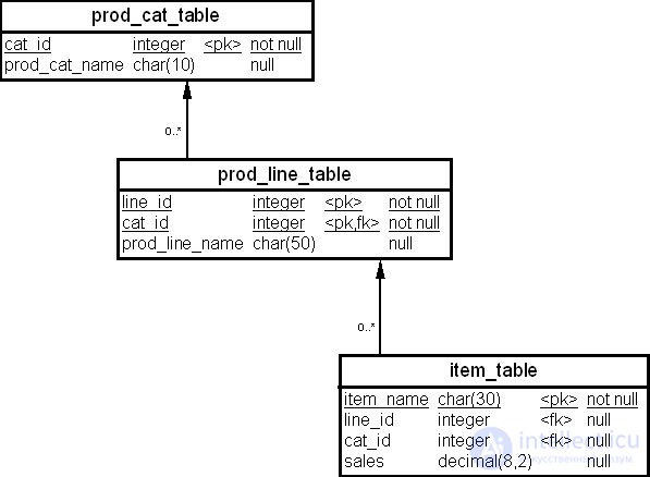
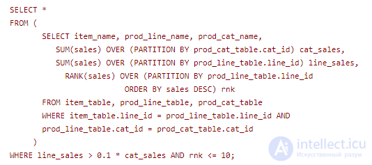
A more complex example is computing the top 10 sales for the product line that contributes more than 10% to the sales of that category. The physical schema for the tables used to solve this problem is shown in Fig. 23.6. The first column is the key for all the tables in the query.

Fig. 23.6. Physical schema for the problem in Example 16.10

CASE expressions and building histograms

The syntax of the CASE statement and some of its applications were discussed in "Designing and Developing the ETL Process". Using the CASE statement, you can easily find the average salary of all employees of an organization (treating any salary below 2000 rubles as equal to 2000 rubles), as shown in the query below:

SELECT AVG(CASE when e.sal > 2000 THEN e.sal ELSE 2000 end) FROM emps e;

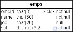
The "Employees" table (emps) includes the columns "Employee ID" (empid), "Full Name" (name), "Job Title" (job), and "Salary" (sal), as shown in Fig. 23.7.

Fig. 23.7. Physical structure of the "Employees" table

The CASE statement can be used to build charts for user-defined buckets (both in terms of the number of buckets and the width of each bucket). In the first example below, a histogram of totals is built across several columns and output as a single row. In the second example, the histogram is shown with a label column and a single column for the totals, output across multiple rows.

Example 23.11. Building a histogram.

Suppose we need to build a histogram of the distribution of customers by age group for elderly people. The age groups are defined by the following conditions: 70-79, 80-89, 90-99, 100+.

The following query solves this problem (assuming that the "Customers" table (customer) contains an "Age" column (age)):

SELECT
SUM(CASE WHEN age BETWEEN 70 AND 79 THEN 1 ELSE 0 END) as "70-79",
SUM(CASE WHEN age BETWEEN 80 AND 89 THEN 1 ELSE 0 END) as "80-89",
SUM(CASE WHEN age BETWEEN 90 AND 99 THEN 1 ELSE 0 END) as "90-99",
SUM(CASE WHEN age > 99 THEN 1 ELSE 0 END) as "100+"
FROM customer;

The result of running the outer query is shown below.

Output 11.

The following query solves the same problem, but outputs the histogram as a "bar."

Example 23.12.

SELECT
CASE WHEN age BETWEEN 70 AND 79 THEN '70-79'
   WHEN age BETWEEN 80 and 89 THEN '80-89'
   WHEN age BETWEEN 90 and 99 THEN '90-99'
   WHEN age > 99 THEN '100+' END) as age_group,
COUNT(*) as age_count
FROM customer
GROUP BY
CASE WHEN age BETWEEN 70 AND 79 THEN '70-79'
   WHEN age BETWEEN 80 and 89 THEN '80-89'
   WHEN age BETWEEN 90 and 99 THEN '90-99'
   WHEN age > 99 THEN '100+' END);

The result of running the outer query is shown below.

Output 12.

Statistical functions in other SQL dialects

In conclusion, it should be noted that some DBMSs have a broader set of statistical functions, window functions, ranking functions, and reporting functions in their SQL dialects. For example, Oracle 11g has a set of functions for building linear regressions.

As an example, let's give a brief overview of the linear regression functions for the Oracle family of DBMSs.

Regression functions fit a regression line to a set of number pairs using the ordinary-least-squares method. These functions are applied to a set of pairs of (e1, e2) after checking all pairs for a zero value (either e1 or e2)l. e1 is the value of the dependent variable (the "y-value"), and e2 is the value of the independent variable (the "x-value"). Both expressions must be numeric. Regression functions are computed in a single pass over all the data.

The list of linear regression functions is given in Table 23.5.

Example 23.13. Computing a linear regression.

In this example, a least-squares regression is computed showing employees' bonuses as a linear function of their salary. The values SLOPE, ICPT, and RSQR are the slope, intercept, and coefficient of determination of the regression, respectively. The values AVGSAL and AVGBONUS are the average salary and average bonus of employees, respectively, and the integer value CNT is the number of employees in the department for which the calculation is performed.

Fig. 23.8. Physical schema of the "Employees" table (Employee)

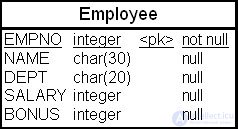
Suppose there is an "Employees" table (Employee) with the columns "Employee ID" (EMPNO), "Full Name" (NAME), "Department" (DEPT), "Salary" (SALARY), and "Bonus" (BONUS) (Fig. 23.8). The table contains eight employees (Table 23.6).

The following query computes the linear regression parameters.

SELECT  REGR_SLOPE(BONUS, SALARY) SLOPE,
        REGR_INTERCEPT(BONUS, SALARY) ICPT,
        REGR_R2(BONUS, SALARY) RSQR,
        REGR_COUNT(BONUS, SALARY) COUNT,
        REGR_AVGX(BONUS, SALARY) AVGSAL,
        REGR_AVGY(BONUS, SALARY) AVGBONUS,
        REGR_SXX(BONUS, SALARY) SXX,
        REGR_SXY(BONUS, SALARY) SXY,
        REGR_SYY(BONUS, SALARY) SXY
FROM employee
GROUP BY dept;

The results of running the query are shown below.

Output 13.

Summary

In this lecture we studied a number of SQL functions used in analytical data processing in data warehouses and data marts. These are statistical functions, ranking functions, and window functions.

Statistical functions perform a calculation over a set of values and return a single value. With the exception of the COUNT function, they ignore NULL values. They are also frequently used in the GROUP BY clause of the SELECT statement.

Ranking functions compute the rank of a record relative to other records in a data set, based on the value of a set of metrics from the data warehouse's fact tables. They return a ranking value for each row in a partition. Depending on the function used, some rows may receive the same rank.

Window functions can be used to compute cumulative, moving, and centered aggregates. They return a value for each row in a table that depends on other rows in the corresponding window. They can only be used in the SELECT and ORDER BY clauses of a query. As a rule, window functions provide access to more than one row of a table without a self-join.

We also examined a number of examples applying the functions listed above to generate reporting data, and, combined with the CASE expression, to build histograms.

It is very useful for a data warehouse designer to know the analytical data processing capabilities of SQL, in order to design data warehouse schemas more effectively and determine the granularity of fact tables.

See also

• data warehouses
• window functions