
Lecture
Dimensional modeling is easier to understand than ER-modeling. Dimensional modeling is a method for modeling and visualizing data as a set of numeric or linguistic indicators or parameters (measures) that describe general aspects of an organization's activity. As a rule, dimensional modeling focuses primarily on numeric data, such as sales figures, balances, profit, weight, or on objects that can be counted, such as articles, patents, books.
Dimensional modeling has much in common with entity-relationship modeling for the relational model, but differs in its goals. The relational model is focused on data integrity and efficiency of data entry. The dimensional model is primarily oriented toward executing complex queries against the database.
The dimensional modeling method is based on the following core concepts: facts, attributes, dimensions, parameters (metrics), hierarchy, granularity.
Fact (fact) — a set of related data elements containing metrics and descriptive data. Each fact typically represents a data element that numerically describes an organization's activity, a business operation, or an event that can be used to analyze the organization's activities or business processes. In a data warehouse, facts are stored in the base tables of the relational database. For example, the price of a product, the number of product units, and so on.
Attribute (Attribute) – a description of a characteristic of a real-world object in the domain. As a rule, an attribute holds a value known in advance that characterizes the fact. Attributes are usually represented as text fields with discrete values. For example, product package dimensions, product odor.
Dimension (dimension) — an interpretation of a fact from some real-world point of view. Like attributes, dimensions contain text values that are strongly related in meaning to one another. Dimensions are usually represented as axes of a multidimensional space, whose points are the facts associated with them. In a dimensional model, each fact is associated with one or more axes. Dimensions typically represent non-numeric, linguistic variables, such as an organization's branches, employees, customers, and so on.
For example, when analyzing sales of products manufactured or sold by an organization, the typical dimensions are time, customers, sellers, and the place of sale or storage of the goods.
Dimensions are defined by enumerating their elements (members). A dimension element (dimensional member) is a unique name or identifier (a linguistic variable) used to define an element's position. For example, the "Time" dimension might contain the following elements: "all months," "quarters," "years."
Dimension elements are often related as "part-whole" or "parent-child", which makes it possible to define one or more hierarchies on the dimension. Each hierarchy can have several hierarchy levels (hierarchy levels). Each dimension element must belong to only one hierarchy level, thereby producing a partition into disjoint subsets. An example is the hierarchy on the "Time" dimension: year, half-years, quarters, months, and days. The "week" dimension element may belong to two months, so a different hierarchy must be defined for it.
A parameter, metric, or measure — a numeric characteristic of a fact that defines the effectiveness of the organization's activity or business action from the point of view of a dimension. As a rule, a metric holds a value of a fact's characteristic that is not known in advance. Specific metric values are described using variables. For example, let a metric be the numeric expression of product sales in monetary terms, the number of product units sold, and so on. A metric is defined via a combination of dimension elements, and thus represents the fact.
Granularity (Granularity) – the level of detail of the data stored in the data warehouse. For example, daily sales volumes.
A dimensional model is visually represented using a cube (or, in the case of more than three dimensions — a hypercube). Let us consider an example. Suppose the sales volume of a trading organization is a function of the variables "Products," "Month," and "Sales Region." Then the dimensions would be "Products," "Time," and "Location." Fig. 9.1 shows a multidimensional data cube representing this function.
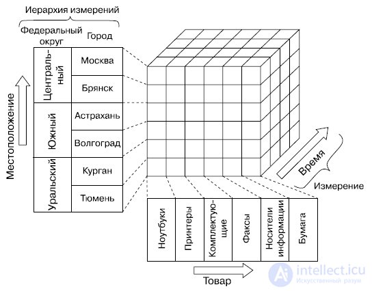
The following hierarchies can be defined on these dimensions:
Dimensional modeling is the primary method of logical design of a data warehouse for OLAP applications. For such applications, drill-up and drill-down operations on data are typical.
Drill down (drill down) and drill up (drill up) are operations that move down and up through the levels of a dimension's hierarchy. When performing a drill-down, the user moves from upper levels to lower levels, which usually contain more detailed data. When performing a drill-up, the user moves from lower hierarchy levels to upper ones, thereby summarizing information at each level. When performing these operations, the navigation path is determined by the dimension hierarchies.
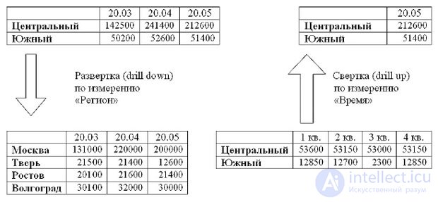
Thus, hierarchies define the paths for summing sales volume. For example, what sales volume of the HP LaserJet 1010 product in the "Printers" category made by HP occurred in week 3 of November in the city of Bryansk at the "Computer Equipment" store.
In order for an application to be able to use these operations for data processing, the data must be arranged in the data warehouse in a certain way, i.e., the dimensional model must be supported.
From the point of view of the relationship between dimensions and facts, the latter can be divided into the following classes:
Let us consider examples of non-additive facts. Facts representing text attributes are non-additive. It makes no sense to sum such facts. For such facts, it makes sense to count their number of occurrences in the fact table. The unit price of a product is also a non-additive fact. It makes no sense to sum the price of an electrical outlet or the unit cost of a product. However, if the product of the unit price and the quantity of goods sold is stored, then this value becomes an additive fact.
Percentages and ratios of quantities (gross margin) are non-additive facts. One can store the numerator and denominator of the ratio as separate parameters, where their separate summation makes sense. These would then be additive facts. Statistical averages, such as the average daily temperature, are also non-additive facts. The sum of average daily temperatures over a week has no meaning whatsoever.
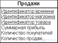
Let us illustrate the concept of an additive fact with an example. Suppose the "Sales" fact table entity (Fig. 9.3), with primary key attributes "Time ID," "Product ID," and "Store ID," has the following facts (metrics): "Number of Customers," "Total Profit," and "Number of Sales." Since summation can be performed for the numeric metrics "Number of Sales" and "Total Profit" of the entity across all dimensions, these facts are additive, as shown in the example below.
Example 9.1. Additive facts can be summed across all dimensions
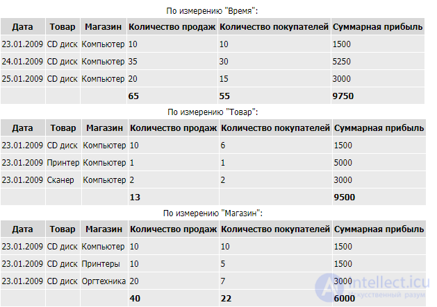
Let us illustrate the concept of a semi-additive fact with an example. Consider the "Sales" fact table entity (Fig. 9.3). As can be seen from example 7.1, summation was not performed for the "Number of Customers" metric along the "Products" dimension, while it was performed along the "Time" and "Store" dimensions. This fact is semi-additive with respect to the "Products" dimension.
Example 9.2. It does not make sense to sum semi-additive facts along certain dimensions
| Date | Product | Store | Number of Sales | Number of Customers | Total Profit |
|---|---|---|---|---|---|
| 23.01.2009 | Fax Paper | Computer | 10 | 6 | 1000 |
| 23.01.2009 | Printer Paper | Computer | 12 | 7 | 1320 |
| 13 |
Example 9.2 shows a table in which the "Number of Customers" metric has been summed along the "Products" dimension. Let us ask the following question: "How many customers bought either printer paper or fax paper?" Answer: somewhere between 5 and 13. The impossibility of splitting the number of customers between products for this entity makes this fact semi-additive for the "Products" dimension.
The primary key in a fact table is, as a rule, a composite primary key. It consists of a set of foreign keys that serve as the primary keys of the dimensions associated with the facts.
It should be noted that sometimes several combinations of foreign keys represent a unique primary key of the fact table. On the other hand, the combination of all the dimension foreign keys does not always guarantee the uniqueness of the fact table's primary key (especially if the fact table contains degenerate dimensions, discussed below in this lecture).
Let us examine the question of the uniqueness of the fact table's primary key in more detail.
Facts are, as a rule, granulated. The granularity of facts determines the semantic meaning of a fact's value from the point of view of the level of detail associated with the fact's information. For example, the total sales volume for a given store on a specified day for a given type of product.
Granularity is often defined at the level of a single business operation. For example, a product sale. Sometimes it is necessary to store information about the sale of a given product per day (here some level of data aggregation is already present).
The uniqueness of the fact table's primary key is guaranteed by the definition of fact granularity, not by the uniqueness condition of the foreign keys from the dimension tables, if the granularity of the facts is not properly defined.
Let us consider the fact table in the diagram of Fig. 9.4. The granularity of the facts in it is one day. Facts are defined for this table as sums over all operations for the day.
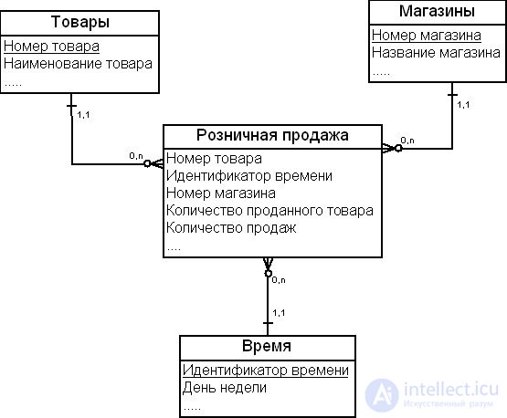
Suppose that the "Products" dimension contains two types of boards — C1 and C2. The "Dates" dimension contains one row per day. Suppose that C1 boards were sold on March 1, 2009, at 9 a.m. in a quantity of 4 units, and in the evening before the store closed in a quantity of 5 units. Since the granularity of the facts is a day, only one row per day will be inserted into the "Retail Sales" fact table for each product sold at each store. Thus, for March 1, 2009, the value 9 will appear in the "Number of Sales" field.
If we define the fact table's primary key as the concatenation of the dimension primary keys {Product Number, Date ID, Store Number}, then this primary key will be unique, since a fact will be a single row inserted for each product sold at each store on a specific day. Uniqueness of the primary key is guaranteed by the definition of fact granularity.
Suppose that the management of a trading company needs reports on hourly product sales. Then the schema shown in Fig. 9.5 could be used.
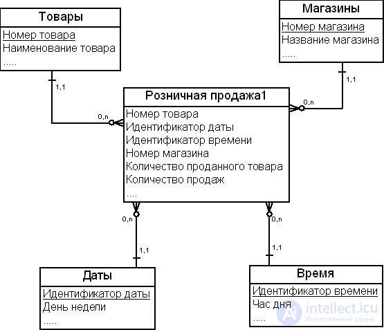
Suppose that on March 12, 2009, C1 boards were sold as follows (Table 9.1).
| Time | Quantity |
|---|---|
| 8-00 | 5 |
| 8-30 | 5 |
| 11-00 | 2 |
| 16-00 | 3 |
| 18-00 | 2 |
Since the granularity of the fact table is one row for each product sold at each store per hour, 4 rows will be inserted into the table, recording the sale of C1 boards for March 2, 2009. If we define the fact table's primary key as the concatenation of the dimension primary keys {Product Number, Time ID, Date ID, Store Number}, then this primary key will be unique.
Thus, the granularity of a fact guarantees the uniqueness of the fact table's composite primary key.
Facts in a dimensional model are conventionally represented in the form of a fact table. In the logical entity-relationship model, the fact table is represented by an entity whose attributes are facts (metrics or descriptions) and a composite key that links the fact table to the dimension tables via a "one-to-many" relationship.
Fact tables are divided into three main categories, depending on the level of detail of the facts (granularity).
The main characteristics of a fact table are as follows.
Thus, a fact table can be divided into two parts. The first part consists of the dimension primary keys, and the second — of the numeric parameters that are functionally dependent on the dimension table keys. A fact table often has a system-generated surrogate primary key, on which, by definition, all the parameters are fully functionally dependent.
An example of a fact table is shown in Fig. 9.3.
The main characteristics of a dimension table are as follows.
Fig. 9.6 shows an example of the "Time" dimension table. "Time ID" is the primary key of the dimension table. The remaining fields are attributes of the fact table parameters that depend on time.
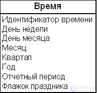
As a rule, a dimension table has a primary key and attributes that describe facts from the perspective of some area of the organization's activity.
There are several schemas for dimensional data modeling. Two of them are considered the primary ones: the star schema (star schema) and the snowflake schema (snowflake schema). In more complex cases, so-called "multi-star" schemas are used, or a schema with multiple fact tables.
The star schema has one fact table and several dimension tables. The dimension tables are denormalized.
The snowflake schema has one fact table and several normalized dimension tables.
The star schema has the same elements as entity-relationship diagrams. These are entities, attributes, primary and foreign keys, relationships, and relationship cardinality.
Fig. 9.7 shows an example of a star schema built for tracking grocery product sales. The "Grocery Sales" fact table (recording grocery sales transactions of a trading company) has one primary key, "Invoice Number," four foreign keys (corresponding to the number of dimensions), and two parameters: "Quantity" (of grocery product sold) and "Product Cost."
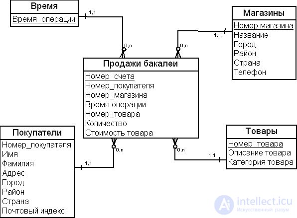
The "Time" dimension is one of the critical elements of a data warehouse model. Whereas in OLTP systems queries focus on the current moment in time, in decision support systems (DSS), for which data warehouses are designed and built, queries focus on data analysis tasks — namely, how data has changed over various periods of time. For example, what was a trading company's sales volume over the last quarter or month, or what are the trends in product purchases over the last quarter.
The "Store" dimension makes it possible to group sales operations by store, taking their geographic location into account.
The "Products" dimension makes it possible to analyze typical purchasing patterns and answer the question of which products are typically bought together by customers.
The "Customers" dimension makes it possible to analyze purchases in terms of frequency, geographic location, and quantity.
Dimension tables serve as a kind of guide when selecting rows from the fact table.
Fact tables have a large number of rows. Dimension tables, as a rule, have far fewer rows. One of the main advantages of using such a schema is that the performance of the DBMS join operation between the fact table and such dimension tables will be close to optimal.
The snowflake schema (Fig. 9.8) adds hierarchy to the dimension tables. For example, the "Region" dimension groups stores by geographic region, the "Product Category" dimension groups products by category, the "Customer Category" dimension groups customers by category, and the "Sales Period" dimension groups sales by time period.
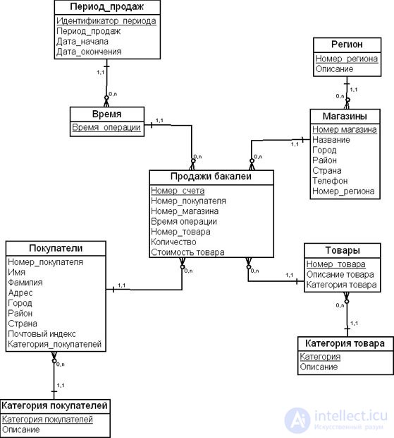
Thus, the use of hierarchies transforms a star schema into a snowflake schema. You can extend snowflake schemas by adding new hierarchies to them, as shown in Fig. 9.9.
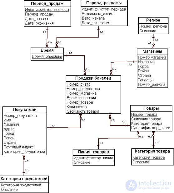
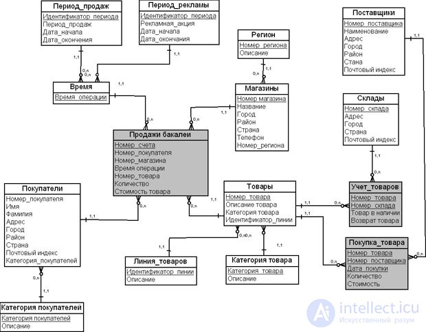
Fig. 9.10 shows an example of a schema with multiple fact tables – the Fact Constellation Schema. This schema has three fact tables: "Grocery Sales," "Inventory," and "Product Purchases," which have both common dimensions ("Products") and exclusive ones (for example, the "Warehouses" dimension for the "Inventory" fact table).
Now let us take a closer look at questions related to modeling dimension tables.
When modeling fact tables, a data warehouse designer primarily relies on considering a characteristic such as the degree of detail (granularity) of the facts.
Above we examined fact tables that contain parameters (metrics) at the lowest level of detail (granularity), such as the level of an organization's business operation, or an instantaneous transaction. An instantaneous transaction provides the ability to register a description of a fact at a specific point in time. These are transactional fact tables. An example of such a table is shown in Fig. 9.3. The "Total Profit," "Number of Sales," and "Number of Customers" facts are recorded in the fact table at the level of a product sale operation (an instantaneous transaction).
Note that such fact tables may contain test attributes and non-additive numeric facts.
An aggregate can be associated with each level of granularity. Aggregates are sums of parameter values, or statistical functions of parameter values, taken at a certain level of detail (granularity). Aggregates on the same facts can be defined at one or more levels of detail.
As a rule, two types of fact aggregate tables are used in a data warehouse, as noted earlier in this lecture:
Aggregates are of great importance for query performance. A query will run much faster on 10 pre-computed rows of a fact table than on ten thousand rows at a lower level of detail.
For example, for the schema in Fig. 9.6, one could build a "daily sales" aggregate by store or region, or a "weekly sales" aggregate by product category.
An aggregate fact table (Aggregate fact table) is a fact table that contains aggregates of certain facts of the model.
The designer adds fact aggregate tables to the dimensional data model and establishes its relationships with the dimensions.
Let us build the "Store Sales" fact aggregate table, containing aggregates of facts on daily store sales, as shown in Fig. 9.11. This table contains total sums for the daily sales of each store.
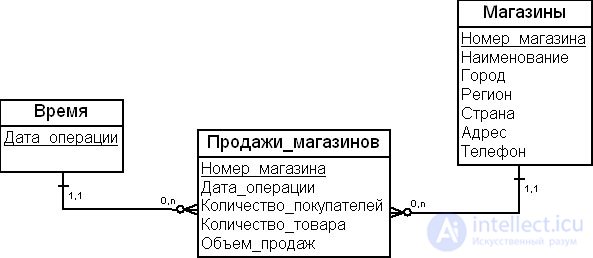
This is an example of a periodic snapshot fact table.
Based on this fact aggregate table, derived aggregates can be built, such as the average number of purchases made by a single customer, or the average amount spent by a single customer on purchases.
The designer can design another fact aggregate table containing data on daily sales by region and product category, as shown in Fig. 9.12.
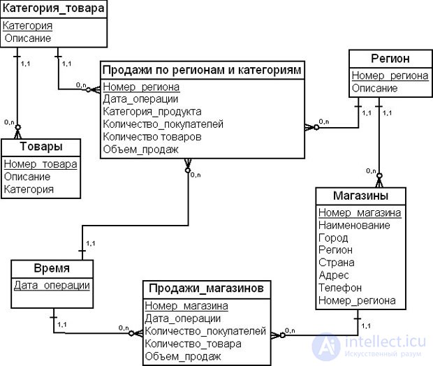
An arbitrary number of fact aggregate tables can be added to a multidimensional data warehouse model. Note that fact aggregate tables represent pre-computed answers to known questions. Unplanned queries against aggregates are generally not supported.
For a fact table associated with 10 dimension tables, there are potentially more than three million possible fact aggregate tables. Which fact aggregate tables should actually be built in the data model depends on the goals of the data warehouse project and on the design decisions made by the data warehouse architect.
When determining aggregates, it is useful to apply the Pareto principle: 20% of the possible aggregate candidates will actually be in demand by users.
A cumulative snapshot fact table aggregates, in a single row of the fact table, data spanning the entire lifetime of some event. For example, a cumulative snapshot fact table might store information about employee payroll cards for some organization. Typically, such cards are issued by a bank for a period of two to five years, after which they are replaced with new cards.
As an example of such an aggregate table, consider a recruitment company. Suppose the company advertises more than 10,000 job openings in the press every day. Management would like to evaluate the effectiveness of its recruiters — namely, how long the candidate hiring process takes, how much time is spent waiting for resumes to arrive, and how much time a company manager spends placing a candidate who has approached the company for its services.
In this fact table, a single row (fact) will contain three time periods for each manager and for each job opening. An example schema is shown in Fig. 9.13.
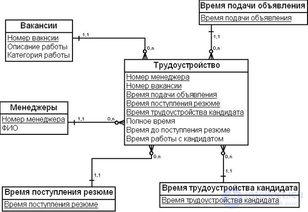
This type of fact aggregate table is generally used for short-lived processes and for processes based on random events, such as a bank transaction.
Table 9.2 provides a comparison of the main types of fact tables.
| Transaction fact table | Periodic snapshot fact table | Cumulative snapshot fact table | |
|---|---|---|---|
| Fact table grain definition | One row per business transaction | One row per period | One row for the entire duration of a completed event |
| Dimensions | Use facts at the lowest level of detail along the "date/time" dimension | Use facts at some aggregated level along the "date/time" dimension (at period end) | Use facts across several "date/time" dimensions to capture results at various checkpoints |
| Total number of dimensions involved | More than in periodic snapshot fact tables | Fewer than in transaction fact tables | The largest number of dimensions among fact table types |
| Facts | Facts are related to operational activity | Facts are related to periodic activity | Facts are related to activity that has a defined lifetime |
| Updates | Not allowed | Not allowed | Allowed |
| Fact table cardinality | Grows quickly | Grows more slowly than transaction fact tables | Grows more slowly than periodic snapshot fact tables |
Now let's turn to the study of dimension modeling.
The values of dimension table fields can change over time. Such changes create problems in dimension table design. This is because data warehouses, by definition and purpose, are intended to store historical data and provide users with access to it.
Slowly Changing Dimensions (SCD) are dimension tables in which some attributes can change their values after a certain period of time, with the frequency of such changes being low.
As an example, consider the "Customer" or "Products" dimension tables. Suppose the primary keys of the tables do not change, while the dimension table attributes can change over time. In that case, three types of actions can be distinguished.
In the first case, the old attribute value is changed to the new value, as shown in the example below. This technique is simple to implement, but it does not allow the history of changes in marital status to be tracked.
Example 9.3. Slowly changing dimensions. Type 1

In the second case, a new record is created in the dimension table with a new surrogate key (Example 9.4). From the perspective of the organization's business operations, a woman who has changed her marital status gets a new employee ID number. Thus, fact table rows "before marriage" will reference the dimension table row with employee ID 332201, and rows "after marriage" – the dimension table row with employee ID 332209.
Example 9.4. Slowly changing dimensions. Type 2
| Employee ID | Last name | First name | Marital status |
|---|---|---|---|
| 332201 | Ivanova | Anna | Single |
| 332209 | Ivanova | Anna | Married |
In the third case, new fields are created in the dimension table to reflect the change in marital status, as shown in Example 7.5 below. As the example shows, two additional fields were needed to preserve the previous marital status and the date it changed.
Example 9.5. Slowly changing dimensions. Type 3
| Employee ID | Last name | First name | Previous marital status | Current marital status | Date of change |
|---|---|---|---|---|---|
| 332201 | Ivanova | Anna | Single | Married | 02.05.2009 |
Let's turn to the schema in Fig. 9.8. Consider the "Customers" dimension. A customer may change their area of residence, and consequently the "City", "Address", and "Zip Code" attributes will change. Suppose the organization analyzes sales facts by region. Then the "Customers" dimension can be classified as type 3. In this case, the "Customers" dimension model needs to be modified, as shown in Fig. 9.14.
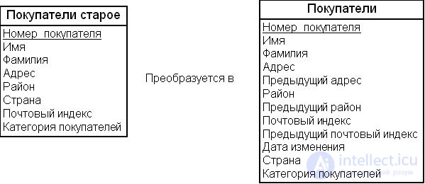
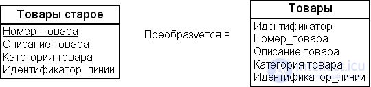
The "Products" dimension in the schema in Fig. 9.8 can be classified as a type 2 slowly changing dimension. An organization may move a product into a different category (for example, when a new product category is created) while keeping a history of changes, i.e. it needs to change the value of the product description attribute. In this case, as described above, a new record is created. Note that if the product number does not change in this case, a surrogate key must be introduced into the dimension, as shown in Fig. 9.15.
The "Product Category" dimension in the schema in Fig. 9.8 can be classified as a type 1 slowly changing dimension. The marketers of a retail organization may refine the description of a product category, and the new description should appear in all reports.
The types listed above characterize slowly changing dimensions almost completely. These types can be combined with one another. A combination of types 1 and 2 is needed when a new record is created for some attributes (type 2), while an existing value is updated for others (type 1). A combination of types 2 and 3 is needed when it is necessary not only to preserve the history of changes by creating a new record (type 2), but also to be able to examine certain facts from the perspective of the historical values of a given dimension record (type 3).
When choosing the type of slowly changing dimension, the data warehouse architect should follow this decision-making scheme:
IF it is required to preserve the dimension's history, THEN choose
type 2.
OTHERWISE
IF it is necessary to compare the current attribute value with the
original or previous one, THEN choose type 3
OTHERWISE
choose type 1.
Surrogate keys are preferable to natural keys (business keys), especially when using type 2.
The values of dimension attributes can change frequently over a short period of time. An example of such a dimension might be the product range of a wire-manufacturing factory. Customers often require wire of a specific diameter to be manufactured. Practice shows that the product range of such factories changes by roughly a third each year.
Rapidly Changing Dimensions are dimension tables in which some attributes can frequently change their values over short periods of time.
The models used to manage such dimensions depend on the cardinality of the dimension tables. If the cardinality of the dimension tables is small (up to 10,000 records), the same approach as for slowly changing dimensions can be used. In the case of very large dimension tables (up to a million records), record duplication should be avoided and no new additional records should be created. Since the performance of queries against such dimensions must be kept in mind, the approaches to modeling such dimensions are important.
As an example of rapidly changing dimensions, consider the "Customers" dimension (Fig. 9.16). For large retail companies, this dimension contains a significant number of records and includes a large number of attributes, including demographic ones. Demographic attributes are often used to study the preferences of different social groups, and customers frequently migrate between social groups.
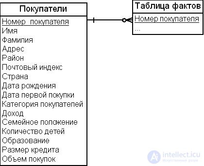
The primary technique for modeling rapidly changing dimensions is to logically split the dimension table into two or more tables. In doing so, a discrete range of values is often used for rapidly changing attributes, in order to reduce the volume of data in the table.
The essence of the logical-splitting technique is as follows: two entities are created, one of which contains the attributes that change slowly, while the other entity includes the attributes that change rapidly. For the "Customers" dimension considered in Fig. 9.16, this can be done as shown in Fig. 9.17 below.
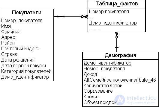
Furthermore, we can assume that a customer's credit operations within the company's retail network will change faster than the rest of the demographic data. In that case, the "Demographics" dimension can be split into two, moving the attributes describing credit and credit purchases into the second dimension.
The advantage of this approach is that frequent changes to a customer's profile do not complicate the data representation and do not increase the memory used, since the schema avoids duplicating the values of slowly changing or unchanging attributes.
Using table splitting also has its drawbacks: in particular, navigating the data will be slower, and applying discrete value ranges to demographic attributes is impractical.
Also note that if the join between the "Customers" and "Demographics" dimensions has low cardinality, then either the fact table will need to be split to make the join more efficient, or a foreign key pointing to the "Customers" dimension will need to be introduced into the "Demographics" dimension, as was done in our example above.
A Degenerate Dimension is a key in a fact table that is not joined to any table, because all the attributes associated with that key reside in other dimensions. This is a dimension without attributes. Typically, a degenerate dimension is represented by the dimension key attributes in the fact table, without a corresponding dimension table.
Degenerate dimensions are often found in fact tables built at a level of detail corresponding to the level of an individual transaction. As a rule, degenerate dimensions are identifiers assigned by operational systems, such as order numbers, credit card transaction numbers, account numbers, invoice numbers, and the like. Degenerate dimensions are the natural keys of the "parents" corresponding to the detail records.
Even though a degenerate dimension is not joined to a table containing additional attributes, it can be useful for grouping related records in the fact table. For example, in Fig. 9.18, for a retail business, the "Receipt Number" attribute groups all products purchased in a single basket, and is a degenerate dimension.
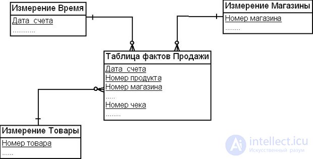
A fact table may have several degenerate dimensions. For example, a fact table for goods shipments may contain both an order number and a shipping invoice number.
Degenerate dimensions can be used to maintain a link to operational systems, and can also be useful during ETL development to relate fact table records to records in operational systems for testing purposes or integrity checks.
The values of degenerate dimensions are typically unique and small in size. However, if a surrogate key is used, say to save memory, or if the operational-system identifier is expressed as a long string, then the dimension is no longer degenerate.
One of the practical criteria for identifying degenerate dimensions (during the operational stage) — the presence of dimension tables whose cardinality grows in proportion to the cardinality of the fact tables. Such dimension tables should be turned into degenerate dimensions.
A hierarchy is an interconnected set of "many-to-one" relationships, consisting of a sequence of levels. For example, the "Region" hierarchy is defined by the levels "Oblast", "District", "City". In other words, a hierarchy is a specification of levels that represent the relationships between different attributes within the hierarchy. As a rule, hierarchies enrich the semantics of relationships between data in a multidimensional model.
In multidimensional modeling, three types of hierarchies are distinguished:
A balanced hierarchy – is a hierarchy in which all branches of the dimension have the same number of levels. For example, the hierarchy "Year" — "Quarter" — "Month". Each level has the same type and is logically equivalent.
A balanced hierarchy consists of a fixed number of levels. The number of attributes in the dimension table corresponds to the number of levels in the hierarchy. Fig. 9.19 shows an example of a balanced "Dates" hierarchy.
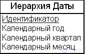
A dimension table can have several hierarchies. For example, the dimension table in Fig. 9.19 could have attributes added for the "Fiscal Year" — "Fiscal Quarter" — "Fiscal Month" hierarchy.
An unbalanced hierarchy – is a hierarchy in which all branches of the dimension have a different number of levels. A "parent-child" type dimension is an example of an unbalanced hierarchy. An organization's structure could be an example of an unbalanced hierarchy: "Director" — "Deputy Directors" — "Departments" — "Laboratories" – "Groups".
The general approach to modeling "parent-child" relationships in relational databases is to introduce the child entity's key into the parent entity. This key is called a recursive pointer. An example of this modeling is shown in Fig. 9.20. The "Manager Number" attribute is a recursive pointer that references "Employee Number".
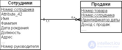
The structure shown in Fig. 9.20 does not work for certain queries. Suppose we need to show the total sales revenue for employee number 2. If employees numbered 5, 4, and 7 report to employee number 2, then we need to show the total sales revenue derived from employees numbered 2, 5, 4, and 7. As a rule, using the GROUP BY clause of a single SELECT statement, it is impossible to sum values down through the levels of the hierarchy. An auxiliary bridge table is used to resolve this situation, as shown in Fig. 9.21.
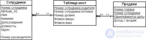
A bridge table is an auxiliary table designed to simplify working with recursive relationships, "many-to-many" relationships, and hierarchy-type relationships within a relational data model.
Let's look at how a bridge table works. The "Employees" dimension table has one row for each employee at every level of the hierarchy. It contains one row for each path in the hierarchy tree — that is, the bridge table contains one row for every path in the hierarchy from an employee to a subordinate reporting to them, as well as a row containing a reference from the employee to themself. In addition, the bridge table contains the hierarchy level number (the number of levels between parent and child in the relationship), a "down" flag indicating that the given employee is at the lowest level of the hierarchy, and an "up" flag indicating that they are at the highest level of the hierarchy.
A bridge table can participate in the join between the "Employees" dimension table and the "Sales" fact table in two ways. When traversing down the hierarchy, the fact table is joined to the bridge table via the "Employee Number" key against the bridge table's "Child Employee Number" key, while the "Employees" dimension table is joined to the bridge table's "Parent Employee Number" via its own "Employee Number" key. The "Level Number" field determines the depth of traversal through the hierarchy. The "Down Flag" field indicates that the lowest level of the unbalanced hierarchy has been reached. When traversing up the hierarchy, the fact table is joined to the bridge table via the "Employee Number" key against the bridge table's "Parent Employee Number" key, while the "Employees" dimension table is joined to the bridge table's "Child Employee Number" via its own "Employee Number" key. The "Level Number" field also determines the depth of traversal through the hierarchy. The "Up Flag" field indicates that the highest level of the unbalanced hierarchy has been reached.
Note that using bridge tables complicates both the design of the data model and its subsequent maintenance. Maintaining such tables typically requires developing packages of stored procedures.
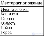
A Ragged hierarchy is a hierarchy in which one of the levels is allowed to be missing when populating it with data, i.e. different variants of the hierarchy are stored within a single data structure.
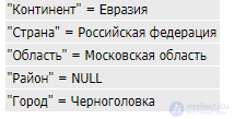
Consider the "Location" dimension table in Fig. 9.22, which represents the geographic location of populated places.
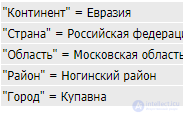
For example, for populated places in the Russian Federation, the dimension table might be populated as follows.
Dimension tables can have "many-to-many" relationships with one another. For example, suppliers may supply goods to different warehouses, and stores may receive goods from various warehouses. A "many-to-many" relationship can exist between: 1) a dimension table and a fact table, 2) between dimension tables.
As a rule, "many-to-many" relationships between database tables are resolved by creating an additional table that manages that relationship (a requirement of fourth normal form in relational database design).
In multidimensional data warehouse modeling, two types of such additional tables can be used to resolve a "many-to-many" relationship between dimension tables: a "empty" fact table, or factless fact table, and a bridge table.
A factless fact table is a fact table that contains no numeric parameters or metrics. A required attribute of this table is a composite key made up of the primary keys of the entities involved in the "many-to-many" relationship. Such fact tables are typically used to represent events or event coverage, and contain information about whether something happened or did not happen.
There are two types of factless fact tables: event tracking tables and coverage tables.
A coverage table describes what has not yet happened — for example, which products have not yet been sold as part of a promotional campaign.
An event tracking table records an event, i.e. the date or time of the event and its description.
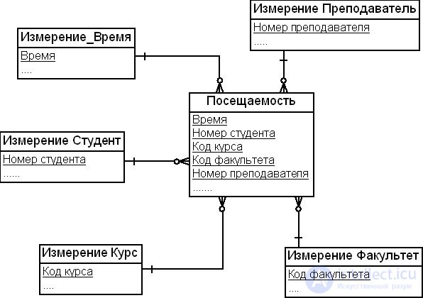
As an example, consider student attendance in courses taught by various instructors. Students at a university study various courses, courses are taught by different instructors, students belong to different faculties, and so on. The entities "Student", "Instructor", "Faculty", "Course", and "Time" are in a "many-to-many" relationship. We can build a factless fact table "Attendance" to track the presence of students from various faculties in courses taught by various instructors, as shown in Fig. 9.23. This resolves the "many-to-many" relationships among the entities (dimensions) discussed above.
A coverage table, also known as an existence table, is typically used when overlapping periods can exist for time-type dimension tables — for example, in a marketing campaign to promote a product to the market involving a flexible pricing grid. In this case, not all stores will be participating in the product promotion at the same time. Nor will all products be part of a given marketing campaign. An example of using a "Stores Products" coverage table is shown in Fig. 9.24.
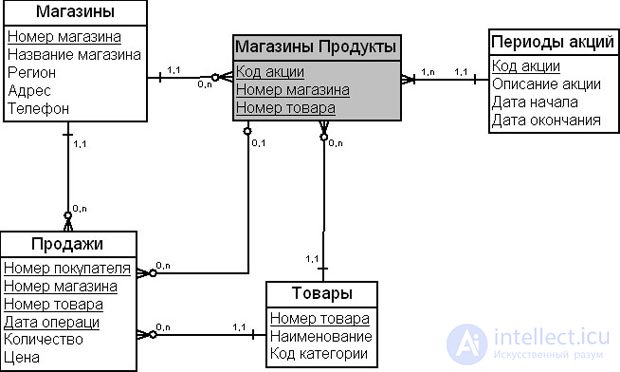
In the example shown in Fig. 9.16a, the coverage fact table is used to determine which product was sold in which store during the period of the marketing campaign.
Such tables should help analysts evaluate the effectiveness of a marketing campaign by identifying the products and stores involved.
In relational modeling, tables that resolve "many-to-many" relationships are called associative tables. Coverage fact tables manage exceptions, where a given entity in one table is related to certain entities in one or more other tables.
The bridge table was defined earlier in this lecture. Recall that a bridge table is an intermediate table that serves to manage the situation associated with implementing multi-valued functional dependencies in data.
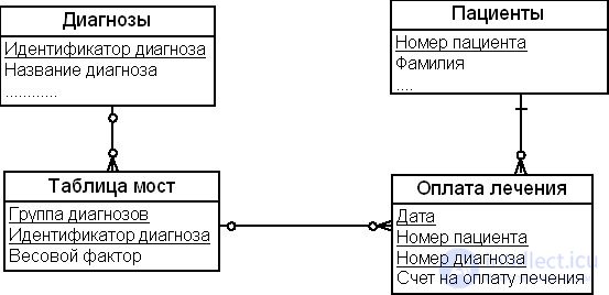
Consider the example in Fig. 9.25, which shows two dimensions: "Patients" and "Diagnoses" – and a "Treatment Payment" fact table, which contains data on treatment payments received against an issued invoice.
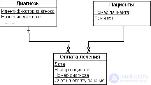
The granularity of the fact table is defined as follows: there is one record about a treatment charge with an established diagnosis per patient. Suppose the treatment of a family that has had a cold is billed on a single invoice. To avoid violating the granularity definition in such cases, we can use a bridge table, as shown in Fig. 9.26.
The "weighting factor" is an important column in the bridge table. We assign a numeric weighting factor to each patient for each family invoice number so that the sum of all weighting factors belonging to an invoice number is exactly 1. The weighting factor is simply a way of distributing numeric additive facts among the patients present in the "Patients" dimension table.
In this lecture we defined and examined the fundamental concepts and elements of the multidimensional model.
The fundamental concepts of the multidimensional model include facts, dimensions, parameters (metrics), and attributes, which are stored in fact tables and dimension tables.
The multidimensional model distinguishes three main types of fact tables:
In the following lectures we will study how these concepts are applied in building data warehouse data models.
The following main schemas are used to represent the multidimensional model:
A number of auxiliary tables are used in the multidimensional modeling process, such as bridge tables and factless fact tables.
The multidimensional model distinguishes the following main dimension tables:

Comments