
Lecture
As already noted in the previous lecture, one of the most important tasks in developing the physical data model of a data warehouse (DW) is ensuring that the DW delivers the required level of performance. In that same lecture we examined the main approach to solving this task — denormalizing the tables of the DW physical data model within the relational model approach. In the present lecture we will continue discussing methods for tackling DW performance and focus our attention on DBMS-specific means for solving this task: indexes, partitions, and clusters.
Indexing — is a way of ensuring fast access to the values of a column or a combination of columns. Physically, new rows are added at the end of the table, resulting in an unordered placement of values within columns. Without some method of ordering the data, the only way for the DBMS to view a column's value is to scan every row sequentially from the beginning of the table to its end — the so-called table scan. The performance of such a scan is proportional to the size of the table, the size of the database's physical page, and the length of the table row.
One way of introducing an ordering relation over column values without disturbing the physical arrangement of table rows is to create a relational DBMS object — an index. An index is an object in a relational database intended to organize fast access to table rows by the values of one or more of their columns.
Conceptually, an index works as follows. It contains an ordered list of values of a column or combination of columns, together with information about the location on disk of the table rows corresponding to those values. The column values in the index are sorted. Even though the order of rows in the table is arbitrary, the index can be scanned quickly to find a specific value. An ordered index can be scanned many times faster than an unordered table. The higher the degree of distinctness of the key values in a column, the faster access to that table's rows will be.
For instance, when a new record is inserted into a table, the primary key's uniqueness check is not implemented by actually scanning the database table, but rather by enforcing a uniqueness requirement on the values of the primary key column within the index. Thus, an index is a database object that can substantially reduce the time needed to find the required rows in a table.
Indexes take up space in the database. When new data is inserted or existing data is deleted, the DBMS has to update both the tables and the indexes. This can slow down data-modification operations, especially for tables with a large number of rows, as is typical in a DW. This gives rise to a conflict between the speed of updating data in a table and the speed of reading it. The following rule of thumb should be followed when resolving this issue: create indexes for primary key columns and other columns frequently used in queries whose data selection relies on logical criteria. If this results in degraded update performance, removing some indexes may be considered.
Every database table can have one or more indexes. Indexes are created on one column or on several columns of a table. The columns included in an index are commonly called key fields, or keys. Indexes can be unique or non-unique. Uniqueness of an index means there are no two rows with the same index key value. A non-unique index can have several keys with identical values.
The main goals of creating indexes in a database are:
At the stage of creating the DW physical data model, a number of important decisions must be made about what and how to index; it is important to clearly formulate indexing rules. For every DW IT project, indexing rules must be developed and documented in writing as part of the overall performance-assurance rules. Maintaining and supporting indexes during DW operation is largely the responsibility of the database administrator. When addressing performance issues, the DBA will raise the question of redesigning the physical structure (reverse design tasks), including the question of dropping and creating new indexes. The DBA may handle these tasks independently. It is therefore all the more important to know by what rules and for what reasons indexes of one type or another were created. Developing such rules will significantly improve the quality of DW operation from a performance standpoint.
To handle these tasks, the designer must know how an index works, what types of indexes the DBMS supports, and understand the meaning of indexing methods.
First we will describe the types of indexes together with the indexing methods for each type, then we will examine how an index works, and finally give some recommendations for creating and using indexes.
An index built on a balanced hierarchical structure (or a B-Tree index, balanced tree structured object) resembles a tree when viewed from the bottom up. When the DBMS works with this structure, it first reads the topmost block — the root node (root), then a block at the next level — a branch block (branch), and so on, until a leaf block (leaf) containing the indexed column(s) of the row is retrieved. Note that the values of the indexed columns are stored in the index (fig. 20.1).
This structure allows the number of I/O operations to be minimized. Obtaining the indexed columns of a row typically requires a single visit to a leaf block, i.e., to the physical page of the database's file structure allocated for the index.
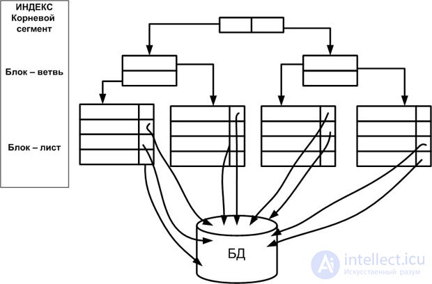
Two cases should be noted in which, after retrieving the indexed columns of a row from the index, several visits to the index's physical page may be required:
A B-Tree index is characterized by the number of levels in the index – its height. The fewer the levels, the higher the performance.
A B-Tree index — is a physical object of a relational database organized on the principle of a balanced hierarchical structure and possessing a set of properties. Let us formulate some properties of B-Tree structured indexes.
In the MS SQL Server family of DBMSs, all indexes are organized on the basis of a balanced hierarchical structure. In addition to having the properties of uniqueness ( UNIQUE ) and non-uniqueness, indexes in the MS SQL Server family can be clustered ( CLUSTERED ) or non-clustered ( NONCLUSTERED ), the latter being the default index type.
A clustered index – is an index in which the logical order of the key values determines the physical order of the corresponding rows in the table. At the bottom (leaf) level of such an index, the table's actual data rows are stored. At any point in time, a table or view can have only one clustered index.
A non-clustered index – is an index that defines a logical ordering for a table. The logical order of rows in a non-clustered index does not affect their physical order. Up to 999 non-clustered indexes can be created for each table, regardless of how they are created: implicitly, via PRIMARY KEY and UNIQUE constraints, or explicitly, via the CREATE INDEX command, which was covered in "Getting to Know the CASE Tool".
In a clustered index, the leaf nodes contain the data pages of the underlying table. The index pages of the root node and intermediate nodes hold index rows. Each index row contains a key value and a pointer either to a page at an intermediate level of the balanced tree, or to a data row at the leaf level of the index. Pages at each level are linked into a doubly linked list.
By default, a clustered index occupies one partition of disk space. If a clustered index spans several partitions, each partition includes a balanced tree containing the data of that partition. For example, if a clustered index spans four partitions, there are four balanced trees: one per partition.
SQL Server descends the index to find the row matching the clustered index key. To find a range of keys, SQL Server first locates the starting key value of the range, and then scans the data pages using the pointers to the next and previous pages. To find the first page in the chain of data pages, SQL Server follows the leftmost pointers from the root of the index.
Depending on the data types, each clustered index structure consists of one or more allocation units, which are used to store and manage the partition's data. For each partition, a clustered index contains at least one IN_ROW_DATA allocation unit. To store large object ( LOB ) columns, a clustered index requires one LOB_DATA allocation unit per partition. In addition, to store variable-length rows that exceed the row-size limit of 8,060 bytes, one ROW_OVERFLOW_DATA allocation unit is required per partition.
In their organization, non-clustered indexes differ from clustered ones as follows: the data rows in the underlying table are not sorted and are stored in an order that is not based on their non-clustered keys; the leaf level of a non-clustered index consists of index pages instead of data pages.
Non-clustered indexes can be defined on a table or view that has a clustered index, or on a heap. Each row of a non-clustered index contains a non-clustered key value and a row pointer. This pointer identifies the data row of the clustered index or heap that contains the key value.
Row pointers in non-clustered index rows are either a row pointer or the clustered index key for the row, as described below.
If a table is a heap (that is, it does not contain a clustered index), then the row pointer is a pointer to the row. The pointer is constructed from a file identifier ( ID ), page number, and row number on the page. The entire pointer is called the row identifier ( RID ).
If the table has a clustered index, or the index is built on an indexed view, then the row pointer is the clustered index key for the row. If the clustered index is not a unique index, SQL Server makes any duplicate keys unique by adding an internally generated value called a uniqueifier. This is a four-byte value invisible to users. It is used whenever the clustered key needs to be made unique for use in non-clustered indexes. SQL Server retrieves the data row by searching the clustered index using the clustered index key stored in the leaf row of the non-clustered index.
By default, a non-clustered index includes one partition. If it consists of several partitions, each partition has a balanced tree structure that contains the index rows for that particular partition. For example, if a non-clustered index contains four partitions, there are four balanced tree structures, one for each partition.
Depending on the data types in a non-clustered index, each of its structures will contain one or more allocation units storing data for a given partition. Each non-clustered index will have at least one IN_ROW_DATA allocation unit per partition, storing the pages of the index's balanced tree. A non-clustered index will also contain one LOB_DATA allocation unit per partition if the index has large object (LOB) type columns. In addition, a non-clustered index will include one ROW_OVERFLOW_DATA allocation unit per partition if the index has variable-length columns that exceed the maximum row size of 8,060 bytes.
Example 20.1.
In the examples that follow, unless stated otherwise, we will use the "Employee" (EMPLOYEE) table (fig. 20.2) from "Designing the DW Model from a Logical Model". Let us repeat it here.
| No. | Attribute name | Column name |
|---|---|---|
| 1 | Personal card number | EMPNO (PK) |
| 2 | Surname | ENAME |
| 3 | First name | LNAME |
| 4 | Department number | DEPNO |
| 5 | Job title | JOB |
| 6 | Date of birth | AGE |
| 7 | Seniority | HIREDATE |
| 8 | Bonuses | COMM |
| 9 | Salary | SAL |
| 10 | Fines | FINE |
| 11 | Biography | Biog |
| 12 | Photo | Foto |
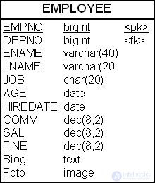
Let us create a composite index on the "Employee" (EMPLOYEE) table for the columns "Surname" (Ename) and "Job" (Job).
CREATE INDEX emp_ndx2 ON EMPLOYEE (Ename, Job)
GO
An index-organized table can be created based on the values of one or more columns. If a query's data requirements can be satisfied from the information contained in the index associated with that data, the underlying table is not accessed.
Some DBMSs, Oracle in particular, support index-organized tables. An index-organized table is a B-Tree type database index that simultaneously serves the role of a table. All of that table's data is stored in the index. The advantage of creating fully indexed tables is savings in disk storage space and a reduction in I/O volume, since the key columns do not need to be stored again in the table. The query result is obtained based on the data stored in the index table.
An index-organized table in Oracle is created using the SQL CREATE TABLE command, as shown in example 20.2.
Example 20.2.
Suppose we need to store and track, in a separate database table, problems arising during the execution of all projects, and also to record who reported them and how often problems occurred. Let us create the index-organized table "Indexed Project" (Proj_Index) to solve this task, as shown below:
CREATE TABLE Proj_Index
( projno	char(8) NOT NULL,
 t_person	char(32) NOT NULL,
t_frequency	integer,
t_problem	varchar2(512),
   CONSTRAINT pk_ndx PRIMARY KEY( projno, t_person) )
ORGANIZATION INDEX
TABLESPACE ts_ndx1
PCTTHRESHOLD 20
INCLUDING   t_frequency
OVERFLOW TABLESPACE ts__of_ndx1;
The CREATE TABLE command is no different from other table-creation commands — until the ORGANIZATION INDEX clause is encountered, which instructs the DBMS to create an index-organized table. A tablespace is specified for placing the index on disk. The PCTTHRESHOLD parameter specifies that the remaining part of the row should be stored in the given tablespace — the overflow segment — if the row exceeds the physical database page size by the given percentage. The INCLUDING parameter defines the name of the column at which the index table row is split into two parts: the index part and the overflow part. This column may be part of the table's primary key or a non-key column. All non-key columns following the specified column are placed in the overflow segment, which is defined by the OVERFLOW keyword.
In the MS SQL Server family of DBMSs there is no built-in capability to create index-organized tables. However, in a number of practical cases, this family of DBMSs allows creating structures analogous to index-organized tables. For this purpose, a non-clustered index with included columns can be used (the INCLUDE option of the CREATE INDEX command).
The INCLUDE option specifies non-key columns to be added at the leaf level of a non-clustered index. A non-clustered index can be unique or non-unique. Column names in the INCLUDE list cannot be repeated and cannot be used simultaneously as key and non-key columns.
For example 20.2, the commands to create a structure similar in purpose to an index-organized table, in the MS SQL Server SQL dialect, look as shown in the example below.
Example 20.3.
First we create the "Indexed Project" (Proj_Index) table, as in fig. 20.3.
CREATE TABLE Proj_Index (
   projno	char(8) NOT NULL,
   t_person	char(32) NOT NULL,
   t_frequency	integer,
   t_problem	varchar(512),
   CONSTRAINT pk_ndx PRIMARY KEY( projno, t_person) )
GO
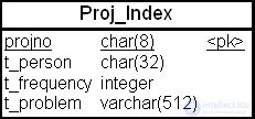
Next, we create a non-clustered index with the key "Project number" (projno) and three non-key columns: "Employee surname" (t_person), "Problem frequency" (t_frequency), and "Problem description" (t_problem).
CREATE NONCLUSTERED INDEX IX_Proj
    ON Proj_Index (projno)
    INCLUDE (t_person, t_frequency, t_problem);
GO
The Oracle DBMS family provides several additional index types that enhance the traditional B-Tree structured indexes common to all DBMSs. Besides index-organized tables, these variants include bitmap indexes, reverse-key indexes, and function-based indexes.
Each bit of a so-called bitmap index corresponds to the row identifier ROWID (which in Oracle is created and stored for every row and used in the internal organization of indexes) in a table object. If a given row contains the key value in question, a one is stored in the index for that value. This organization can, in some cases, significantly improve query performance, since to retrieve rows with particular index values the DBMS need only find all the ones matching the key. Physically, such an index is organized on the basis of a B-Tree structure, but the task reduces to finding the given row through a single read of the bitmap index structure. This index type is very effective for indexing columns with low cardinality — gender, color, and so on. If a column has many distinct values, the amount of I/O will increase.
Example 20.4.
For our study example, we can build a bitmap index on the "Employee" (EMPLOYEE) table for the "Department number" (DEPNO) column:
CREATE BITMAP INDEX emp_ndx ON EMPLOYEE (DEPNO);
In the MS SQL Server family of DBMSs, there is no capability to create bitmap indexes using the SQL dialect.
A reverse-key index applies byte reversal to the values of a numeric indexed column. This technique allows column values to be distributed evenly among the leaf blocks of a B-Tree structured index, which works well for indexing columns with sequential numbering or numbering with a fixed step. Note that such indexes are used only for returning individual rows, and cannot be used to search for values within a range. In Oracle, the REVERSE option cannot be applied to bitmap indexes or to index-organized tables.
Example 20.5.
Numeric keys containing sequential numbers exist, in particular, in the "Employee" (EMPLOYEE) table – "Employee number" (EMPNO). We can create an additional reverse-key index for this table to retrieve an employee's record. Note that a primary key index already exists for this column.
CREATE INDEX dep_ndx ON EMPLOYEE (EMPNO) REVERSE;
During operation, the database administrator can rebuild this index using the ALTER INDEX command:
ALTER INDEX EMPLOYEE REBUILD NOREVERSE;
In the MS SQL Server family of DBMSs, there is no capability to create reverse-key indexes using the SQL dialect.
If a function is applied to an indexed column in a WHERE clause, the DBMS usually does not use that index when organizing access to the table's rows. But when a function-based index is created using the same function as in the WHERE clause, both the Oracle and MS SQL Server families of DBMSs use such an index to read the rows satisfying the selection criterion.
In the MS SQL Server family of DBMSs, computed columns can have the PERSISTED property. This means the Database Engine stores the computed values in the table and updates them whenever any columns on which the computed column depends are updated. The Database Engine uses these materialized values when it builds an index on the column and when a query accesses the index.
For a computed column to be indexable, it must be deterministic and precise. If the PERSISTED property is used, the list of indexable computed column types is extended to include the following types:
Example 20.6.
As an example of using indexes on a computed column, let us look at an example of simulating a hash index in MS SQL Server.
Suppose no index has been created for the "Surname" (ENAME) column in the "Employee" (EMPLOYEE) table. Then, if the WHERE clause of a SELECT command specifies a search predicate on the "Surname" (ENAME) column, the DBMS will scan the table. If the table contains around 1,000,000 rows, the scan operation will increase the query's processing time.
Let us create a hash index for the "Surname" (ENAME) column using the checksum() function; to do this, we add a computed column to the table, as shown below.
alter table EMPLOYEE
add ENameHash as checksum(EName);
go
Next let us create an index on this column, as shown below.
create index IDX_ENames on EMPLOYEE (ENameHash);
go
With such an index present in the database, the DBMS will use it when processing the query described in this example.
In the MS SQL Server family of DBMSs, filtered indexes can be created and used; to create such indexes, the CREATE INDEX command provides the option of using a WHERE clause.
Using a WHERE
The filter predicate uses simple comparison logic and cannot reference a computed column, a user-defined type column, a spatial data type column, or a hierarchyID type column. Comparisons using NULL literals with comparison operators are not allowed. Instead, the IS NULL and IS NOT NULL operators are used.
A filtered index is well suited for columns with clearly defined subsets of data.
Example 20.7.
Let us create a filtered index on the "Employee" (EMPLOYEE) table for the "Fines" (FINE) column, to quickly retrieve lists of fined employees.
CREATE NONCLUSTERED INDEX IDX_FINE
    ON EMPLOYEE (EName, FINE)
    WHERE FINE > 0;
GO
In this section we examined various types of indexes and examples of their creation. In the next section we will look in more detail at index design parameters.
When designing indexes, one needs some mechanism for evaluating the quality of a prospective index. Let us introduce a few concepts that can be used to roughly assess the quality of a potential index.
A table column's cardinality is the number of discrete distinct values of the column that occur in the table's rows. For example, if in the "Employee" (EMPLOYEE) table we add a column to indicate gender – "Sex" (SEX) – then this column's cardinality is 2, since in nature people have only two sexes — male and female. For a primary key column, the cardinality equals the number of rows in the table.
The reason column cardinality matters for index design is that the cardinality of an indexed column determines the number of unique entries that must be stored in the index, i.e. the number of records in the index. For example, the indexed column "Sex" (SEX) will have only two unique entries, each of which will be repeated many times in the index. Assuming an equal distribution of employee sex over 100,000 rows in the "Employee" (EMPLOYEE) table, each index entry will be repeated 50,000 times. A DBMS is unlikely to choose to use such an index when building a query plan.
Determining the cardinality of a potential indexing column in an existing database table is quite simple.
SELECT COUNT (DISTINCT колонка) FROM таблица;
When designing a new data warehouse database, the cardinality of all potential indexed columns in all tables of the data warehouse's physical data model should be estimated based on the available documentation.
The way a DBMS evaluates the effect of cardinality is by using the selectivity factor. The selectivity factor of an index is defined as the inverse of the cardinality of the indexed column:

The selectivity factor estimates the potential volume of I/O operations. The smaller the selectivity factor, the fewer I/O operations are required to obtain the result set of table rows. The DBMS evaluates this value to decide whether or not to use an index to access the table's rows.
To conclude this section, let us list rules for identifying columns that are good and bad candidates for indexing. These rules can be used when deciding on building indexes for a relational database.
Good candidates for indexing are generally:
Factors that reduce index effectiveness:
Bad candidates for indexing are generally:
продолжение следует...
Часть 1 Designing data warehouse performance — indexing
Часть 2 Improving query performance: partitioning - Designing data warehouse performance —
Часть 3 Improving query performance: clusters - Designing data warehouse performance —
Часть 4 Summary - Designing data warehouse performance — indexing

Comments