
Lecture
Это продолжение увлекательной статьи про повышение производительности запросов.
...
via the index causes many table pages to be visited many times over;
The following general rules should be observed when creating indexes.
Unfortunately, designers often make extremely poor indexing decisions. This results in a data warehouse with far too many indexes. As a result, a great deal of time is spent maintaining these indexes, disk space is used inefficiently, and the DBMS becomes "confused" when choosing a suitable index, or does not use them at all. Therefore, it is important to keep in mind the two fundamental principles of index design:
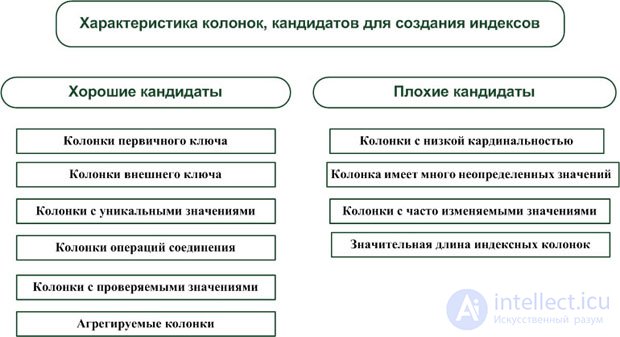
Fig. 20.4 shows recommendations for selecting columns for creating indexes.
As a rule, data warehouse tables contain a huge amount of data. The larger the table, the more time is required for certain row-retrieval operations and for certain database administration tasks — for example, backup and recovery. Large indexed tables also have large indexes, which require a great deal of DBMS time to maintain.
Partitioning is a way of physically distributing tables and indexes among two or more tablespaces (Oracle DBMS) or one or more filegroups (MS SQL Server DBMS), depending on the values of the tables' key columns, for the purpose of improving I/O performance. Thus, partitioning is the division of a table into groups while preserving a common structure definition across all the groups. A tablespace (Oracle DBMS) or filegroup (MS SQL Server DBMS) is the physical location of database tables within the operating system's file structure.
A fragment of a table located in a separate filegroup will be called a table partition. Partitioning also improves the efficiency of backup and recovery, since these tasks are performed on a smaller volume of data. A table partition can be thought of as a predefined, named chunk of storage on one or more disks that can be referenced by name in SQL statements.
One important concept in implementing partitioning is the table column whose values the DBMS uses to physically distribute the table across the various filegroups on the hard disks. This column is called the partition key.
Partitioning of tables and indexes is fixed at the row level (partitioning by columns is not allowed) and allows access through a single entry point (the table name or index name), such that application code does not need to know the number of partitions behind that entry point. Partitioning can be applied to the base table as well as to its associated indexes.
We will examine table partitioning separately for the Oracle and MS SQL Server DBMS families.
The Oracle DBMS family supports several types of partitioning: range partitioning, hash partitioning, composite partitioning, and various types of index partitioning.
Range partitioning means distributing a table's rows across different predefined tablespaces depending on the value of the partition key. Such a table, like any other, is accessed by its name, and partitions located in each tablespace can be accessed separately. For example, a table holding an organization's quarterly financial reports could be partitioned by date so that each quarter's reports are stored in a separate tablespace. With this partition layout, only data for a single quarter will be selected from a single tablespace, which improves the overall efficiency of the database.
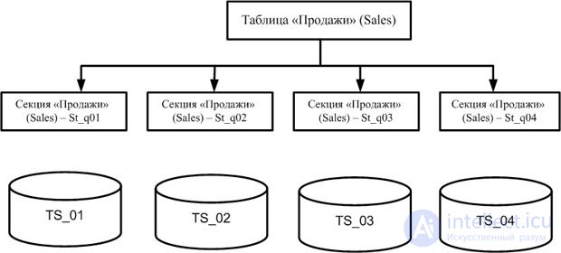
Range partitioning is based on ordering a table's rows into partitions according to the value of the partition key column. Conceptually, a table partitioned by range is structured as shown in Fig. 20.5.
To create partitioned tables, the SQL command CREATE TABLE is used together with the PARTITION clause. In Oracle DBMS, the partition key cannot be of type LONG.
Example 20.8.
Consider an order-processing system. Suppose it has a "Sales" table that stores data about the quantity, time, and price of sales for each customer. Range partitioning — specifically, partitioning by quarter — can be used to represent this table in the database. Suppose we have four previously defined tablespaces named ts_01, ts_02, ts_03, ts_04, distributed across four disks, as shown in the figure below.
The following script fragment defines the "Sales" table with the physical partition layout shown in Fig. 20.5:
CREATE TABLE Sales
(
s_customer_id		number(6),
s_amt			number(9,2),
s_date			date)
PARTITION BY RANGE (s_date)
     (PARTITION st_q01 VALUES LESS THAN ('01-apr-2002')
	TABLESPACE ts_01,
     PARTITION st_q02 VALUES LESS THAN ('01-jul-2002')
	TABLESPACE ts_02,
     PARTITION st_q03 VALUES LESS THAN ('01-oct-2002')
	TABLESPACE ts_03,
     PARTITION st_q04 VALUES LESS THAN (MAXVALUE)
	TABLESPACE ts_04
);
The PARTITION BY RANGE (s_date) clause instructs Oracle DBMS to partition the table by the partition key s_date. Clauses such as (PARTITION st_q01 VALUES LESS THAN ('01-apr-2002') TABLESPACE ts_01 define the partition name st_q01 and its placement in the corresponding tablespace ts_01.
To access the table rows located in a particular partition, and to find out about sales in the third quarter, you can use the SELECT command as shown below:
SELECT s_customer_id, s_amt FROM Sales PARTITION (st_q03);
We see that in order to access the rows of a table partition, you need to specify the PARTITION (partition name) option after the table name in the FROM clause.
A database administrator can easily drop, add, move, split, truncate, and modify partitions using the ALTER TABLE command. An individual partition can also be dropped by dropping the corresponding tablespace.
Hash partitioning means evenly distributing a table's rows across the assigned tablespaces depending on the value of the partition key, which in this case is hashed. This type of partitioning is convenient to use for rows whose partition key value distribution is uneven or hard to group. To decide whether to create a hash-partitioned table, you need a fairly accurate estimate of the table's size, since Oracle DBMS's built-in hashing algorithms use this size to compute the row's position on a physical database page. An inaccurate estimate of table size can lead to a large number of collisions, i.e. rows with different key values landing on the same page, which requires maintaining overflow chains and causes additional I/O.
Example 20.9.
Consider the same "Sales" table as in example 20.8, and the same tablespace scheme (Fig. 20.5). However, let us use "Customer ID" (s_customer_id) as the partition key. Note that the distribution of this column's values may be very uneven. A fragment of SQL code for creating the hash-partitioned "Sales" table can be written as follows:
CREATE TABLE Sales
(
s_customer_id		number(6),
s_amt			number(9,2),
s_date			date)
PARTITION BY HASH (s_customer_id)
     (PARTITION q01 TABLESPACE ts_01,
     PARTITION q02 TABLESPACE ts_02,
     PARTITION q03  TABLESPACE ts_03,
     PARTITION q04 TABLESPACE ts_04
);
The PARTITION BY HASH (s_customer_id) clause instructs Oracle DBMS to partition the table by the partition key s_customer_id. Clauses such as (PARTITION q01 TABLESPACE ts_01 define the partition name st_q01 and its placement in the corresponding tablespace ts_01.
Composite partitioning is a combination of range partitioning and hash partitioning. This means the table is first distributed across tablespaces based on ranges of the partition key value, then each of the resulting range partitions is divided into subordinate partitions, or subpartitions, and the rows are then evenly distributed among the subpartitions by the hash-key value.
Example 20.10.
Consider the same "Sales" table as in the previous example, with the same tablespace scheme. We will use the "Sale Date" column (s_date) as the range partitioning key, and "Customer ID" (s_customer_id) as the hash partitioning key. However, now each range partition will be split into a predefined number of subpartitions. A fragment of SQL code for creating the composite-partitioned "Sales" table can be written as follows:
CREATE TABLE Sales
(
s_customer_id		number(6),
s_amt			number(9,2),
s_date			date)
PARTITION BY RANGE (s_date)
SUB PARTITION BY HASH (s_customer_id)
SUB PARTITION 4
STORE IN (ts_01, ts_02, ts_03, ts_04)
     (PARTITION q01 VALUES LESS THAN ('01-apr-2002'),
     PARTITION q02 VALUES LESS THAN ('01-jul-2002'),
     PARTITION q03 VALUES LESS THAN ('01-oct-2002'),
     PARTITION q04 VALUES LESS THAN (MAXVALUE)
);
Partitions q01, q02, q03, q04 will contain rows within the date ranges defined in clauses such as PARTITION q02 VALUES LESS THAN ('01-jul-2002'), and will be distributed across the tablespaces ts_01, ts_02, ts_03, ts_04. The SUB PARTITION 4 clause instructs Oracle DBMS to split each partition into four logical units, while the SUB PARTITION BY HASH (s_customer_id) clause distributes the rows of a given range among these four subordinate partitions.
Oracle DBMS provides for index partitioning, which means deliberately distributing table indexes among assigned tablespaces according to the partition key. Index partitioning can be global or local.
A locally partitioned index has the same partition key, the same number of tablespaces, and the same partitioning rules as its corresponding base table. A globally partitioned index contains a PARTITION BY RANGE clause that specifies partitioning parameters different from those of the corresponding base table.
Partitioned indexes can be prefixed or non-prefixed. In the case of a prefixed partitioned index, partitioning is performed on the partition key, which contains the leading part of the index key. In the case of non-prefixed partitioned indexes, partitioning is performed on values other than the values of the indexed column.
Indexes can be partitioned even when the indexed table itself is not partitioned. In this case, the index is assumed by default to be a globally partitioned index. Oracle DBMS does not support globally partitioned non-prefixed indexes.
In a locally partitioned index, the key values of one index partition correspond to rows of the table from a single table partition.
Example 14/11.
Let us create a locally partitioned index for the "Sales" table from example 20.8. The partition key of this table is the "Sale Date" column (s_date). A fragment of the index creation code is given below:
CREATE INDEX sales_ndx ON Sales (s_date)
LOCAL
(PARTITION st_i_q01 TABLESPACE ts_01,
     PARTITION st_i_q02 TABLESPACE ts_02,
     PARTITION st_i_q03 TABLESPACE ts_03,
     PARTITION st_i_q04  TABLESPACE ts_04
);
A locally partitioned index is called equi-partitioned if it has the same number of partitions and the same partitioning rules as its base table. Note that this example's index creation did not use the PARTITION BY RANGE clause. Oracle DBMS automatically derives the partitioning structure for the index from the partitioning structure of the base table Sales. It is also possible to omit clauses such as PARTITION st_i_q02 TABLESPACE ts_02. If PARTITION is omitted, Oracle DBMS will automatically generate partition names. If TABLESPACE is omitted, Oracle DBMS will automatically place the partitions in the same tablespaces as the corresponding partitions of the base table.
A globally partitioned index has a partition structure that differs from the partition structure of this index's base table. As an example, let us create a globally partitioned index for the "Sales" table from example 20.8.
Example 20.12.
Let us take the "Customer ID" column (s_customer_id) as the partition key for the index. In the code fragment below, the index partitions use other index tablespaces named ts_i_01, ts_i_02, ts_i_03. The number of index partitions does not match the number of base table partitions for this index.
CREATE INDEX sales_ndx ON Sales (s_customer_id)
GLOBAL
PARTITION BY RANGE (s_customer_id)
(PARTITION st_i_q1 VALUES LESS THAN (10000)
TABLESPACE ts_i_01,
     PARTITION st_i_q2 VALUES LESS THAN (20000)
TABLESPACE ts_i_02,
     PARTITION st_i_q3 VALUES LESS THAN (MAXVALUE)
TABLESPACE ts_i_03,
);
A locally partitioned index can be created on a column other than the base table's partition key. In example 20.13, such a non-prefixed index is created for the "Sales" table from example 20.8.
Example 20.13.
The "Customer ID" column (s_customer_id) is used as the partitioning column for the index, and different tablespaces are chosen for the index partitions — ts_i_01, ts_i_02, ts_i_03, ts_i_04 — which differ from the tablespaces of the base table's partitions for this index.
CREATE INDEX sales_ndx_1 ON Sales (s_customer_id)
LOCAL
(PARTITION st_i_q01 TABLESPACE ts_i_01,
     PARTITION st_i_q02 TABLESPACE ts_i_02,
     PARTITION st_i_q03 TABLESPACE ts_i_03,
     PARTITION st_i_q04  TABLESPACE ts_i_04
);
When deciding whether to partition indexes, the following should be kept in mind.
Oracle DBMS provides the ability to partition views. The basic idea behind view partitioning is simple. Suppose a physical table is split into several tables (not necessarily using table partitioning methods) according to a splitting criterion that makes query processing more efficient. We will call this splitting criterion the partitioning predicate. Views can then be created and configured so that accessing the data in these tables is simpler for the user. A view partition is defined according to a range of partition key values. Queries that use a range of values to retrieve data from view partitions will only access the partitions that correspond to the ranges of the partition key values.
View partitions can be defined by partitioning predicates specified either using a CHECK constraint or using a WHERE clause. Let us show how both approaches can be applied, using a slightly modified version of the "Sales" table we examined in the previous section. Suppose the sales data for a calendar year are stored in four separate tables, each corresponding to a quarter of the year — Q1_Sales, Q2_Sales, Q3_Sales, and Q4_Sales.
Example 20.14.
View partitioning using a CHECK constraint. Using the ALTER TABLE command, you can add constraints on the "Sale Date" column (s_date) of each table so that its rows correspond to one of the year's quarters. The sales view created afterward then makes it possible to query these tables either individually or all together.
ALTER TABLE Q1_Sales ADD CONSTRAINT C0 CHECK (s_date BETWEEN 'jan-1-2002' AND 'mar-31-2002');
ALTER TABLE Q2_Sales ADD CONSTRAINT C1 CHECK (s_date BETWEEN 'apr 1-2002' AND 'jun-30-2002');
ALTER TABLE Q3_Sales ADD CONSTRAINT C2 check (s_date BETWEEN   'jul-1-2002' AND 'sep-30-2002');
ALTER TABLE Q4_Sales ADD CONSTRAINT C3 check (s_date BETWEEN   'oct-1-2002' AND 'dec-31-2002');

CREATE VIEW sales_v AS
  SELECT * FROM Q1_Sales UNION ALL
  SELECT * FROM Q2_Sales UNION ALL
  SELECT * FROM Q3_Sales UNION ALL
  SELECT * FROM Q4_Sales;
The advantage of this kind of view partitioning is that the CHECK constraint predicate is not evaluated for every row of the query. Such predicates prevent rows that do not meet the predicate's criterion from being inserted into the tables. Rows matching the partitioning predicate are retrieved from the database faster.
Example 20.15.
View partitioning using a WHERE clause. Let us create a view for the same tables as in the example above.
CREATE VIEW sales_v AS
  SELECT * FROM Q1_Sales WHERE s_date BETWEEN  'jan-1-2002' AND 'mar-31-2002'
UNION ALL
  SELECT * FROM Q2_Sales WHERE s_date BETWEEN  'apr-1-2002' AND 'jun-30-2002'
UNION ALL
  SELECT * FROM Q3_Sales WHERE s_date BETWEEN 'jul-1-2002' AND 'sep-30-2002'
UNION ALL
  SELECT * FROM Q4_Sales WHERE s_date BETWEEN 'oct-1-2002' AND 'dec-31-2002';
The method of view partitioning using a WHERE clause has some drawbacks. First, the partitioning criterion is evaluated at runtime for every row in every partition touched by the query. Second, users can mistakenly insert a row into the wrong partition — for example, insert a row belonging to the first quarter into the third quarter — which will lead to incorrect data retrieval for those quarters.
This approach does have an advantage over using a CHECK constraint. A partition corresponding to a WHERE predicate can be placed on a remote database. A fragment of the view definition is given below.
SELECT * FROM east_sales@icp.ac.ru WHERE LOC = 'EAST'
UNION ALL
SELECT * FROM west_sales@ioc.ac.ru WHERE LOC = 'WEST';
When deciding whether to create partitioned views, keep the following factors in mind.
The MS SQL Server DBMS family also supports partitioning of tables, indexes, and views. However, unlike the Oracle DBMS family, partitioning in the MS SQL Server DBMS family is implemented using a unified scheme.
In MS SQL Server, all tables and indexes in a database are considered partitioned, even if they consist of just a single partition. In fact, partitions represent the basic organizational unit in the physical architecture of tables and indexes. This means that the logical and physical architecture of tables and indexes that include several partitions fully mirrors the architecture of tables and indexes that consist of a single partition.
Partitioning of tables and indexes is fixed at the row level (partitioning by columns is not allowed) and allows access through a single entry point (the table name or index name), such that the application code does not need to know the number of partitions. Partitioning can be applied to the base table as well as to its associated indexes.
To create a partitioned table in MS SQL Server DBMS, the following database objects are used: partition functions and partition schemes. These objects make it possible to split data into specific segments and control their location within the database or data warehouse. For example, data can be distributed across several disk arrays depending on the date the data arrived, or other distinguishing characteristics. Note that a table can be partitioned by one of its columns, and each partition must contain data that cannot be stored in other partitions.
When partitioning a table, you first need to define the rule by which the data will be split into segments. Matching individual rows of data to different segments is the job of a partition function.
Data rows can be segmented by a column of any type except the following: text, ntext, image, xml, timestamp, varchar(max), nvarchar(max), varbinary(max), data type aliases, and CLR user-defined types. However, the partition function must assign each data row to only one partition of the table; in other words, as a result of applying the function, the same row cannot belong to several partitions at once.
To partition a table, you need to create or choose a partitioning column (the partition key) in it. The partition key can be created in the table schema when the table is created, or added later by modifying the table. The column can accept NULL values, but all rows containing NULL values will, by default, be placed in the leftmost partition of the table. This can be avoided by specifying, when creating the partition function, that NULL values should be placed in the rightmost partition of the table. The choice between the left and right partitions is an important design decision that becomes apparent when the partition scheme is changed, when additional partitions are added, or when existing ones are removed.
When creating a partition function, you can choose the LEFT or RIGHT functions. The difference between LEFT and RIGHT partitions lies in how the data is distributed across the partitions. The LEFT function distributes data from the lowest value to the highest value (that is, in ascending order). The RIGHT function distributes data from the highest value to the lowest (that is, in descending order). Let's look at an example.
Example 20.16.
Consider the following examples of defining partition functions using LEFT and RIGHT:
CREATE PARTITION FUNCTION Left_Partition (int) AS RANGE LEFT
FOR VALUES (1,10,100)

CREATE PARTITION FUNCTION Right_Partition (int) AS RANGE RIGHT
FOR VALUES (1,10,100)
In the first function ( Left_Partition ), the values 1, 10, and 100 are placed in the first, second, and third partitions respectively. In the second function ( Right_Partition ), these values are placed in the second, third, and fourth partitions.
When creating a partitioned table, it is important for the partitions to be balanced by cardinality. This makes it possible to estimate how much disk space each partition will require. Using the LEFT and RIGHT parameters determines where the data will be placed, which in turn determines the size of the partition and the size of the indexes created on it.
You can determine the number of the partition into which particular data will fall using the $PARTITION function, as shown below:
SELECT $PARTITION.Left_Partition (10)
SELECT $PARTITION.Right_Partition (10)
The first SELECT command returns the value 2, the second returns the value 3.
After creating the partition function and choosing how to split data across partitions, you need to decide where each partition will be created in the file system. Partition schemes are used to establish the link between partitions and their placement in the file system. Partition schemes control how individual partitions are stored on disk by using filegroups to place each partition on the disk subsystem. Partition schemes can be configured so that all partitions reside in a single filegroup, so that each partition resides in its own filegroup, or so that several partitions share common filegroups. The last approach gives the database administrator wide latitude in spreading disk I/O operations around.
Example 20.17 shows some of the ways you can assign one or more filegroups to a partition scheme. Keep in mind that the filegroups used by a partition scheme must already exist in the database before the scheme is created.
Example 20.17.
Let's assign filegroups to a partition scheme. First, here is an example of placing all partitions of a table in a single filegroup named PRIMARY.
CREATE PARTITION SCHEME Primary_Left_Scheme
AS PARTITION Left_Partition
      ALL TO ([PRIMARY])
To place all partitions in different filegroups, run the following command:
CREATE PARTITION SCHEME Different_Left_Scheme
AS PARTITION Left_Partition
      TO (Filegroup1, Filegroup2, Filegroup3, Filegroup4)
To place several partitions in different filegroups, run the following command:
CREATE PARTITION SCHEME Multiple_Left_Scheme
AS PARTITION Left_Partition
      TO (Filegroup1, Filegroup2, Filegroup1, Filegroup2)
If you create the partition functions specified in the example and use the given partition scheme to create the table, you will subsequently be able to determine where individual data rows will be placed in the partitioned tables.
Example 20.18.
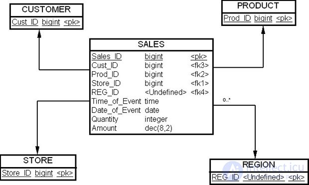
Let's consider, as an example, a star schema with the "Sales" (SALES) fact table, as shown in Fig. 20.6. Let's create a partitioned "Sales" (SALES) table.
First, we need to create a partition function:
CREATE PARTITION FUNCTION
  MyPartitionFunctionLeft
  (date)
  AS RANGE LEFT
  FOR VALUES ('1/01/2005', '1/01/2007', '1/01/2009)
MyPartitionFunctionLeft is the name of the partition function, datetime is the data type of the partition key, and RANGE LEFT specifies how to split the data values associated with the dates in FOR VALUES.
The partition key has the data type date, i.e. it is the "Event date" (Date_of_Event) column. In the command above, rows are split into non-overlapping groups on the principle of dividing them into two-year groups. Splitting into
продолжение следует...
Часть 1 Designing data warehouse performance — indexing
Часть 2 Improving query performance: partitioning - Designing data warehouse performance —
Часть 3 Improving query performance: clusters - Designing data warehouse performance —
Часть 4 Summary - Designing data warehouse performance — indexing

Comments