
Lecture
Это продолжение увлекательной статьи про повышение производительности запросов.
...
style="color:rgb(139, 0, 0); font-family:monospace">RANGE LEFT partitions divides the data into the value ranges shown in Fig. 20.7.

Each range of values in a partition has boundaries that are defined in the FOR VALUES clause. If a sale date was June 23, 2006, the row will be stored in partition 2 (P2).
Now let's create the partition scheme. The partition scheme maps partitions to different filegroups (named MyFilegroup1, MyFilegroup2, MyFilegroup3, MyFilegroup4 ), as shown in the following command:
CREATE PARTITION SCHEME
  MyPartitionScheme
  AS MyPartitionFunction
  TO (MyFilegroup1, MyFilegroup2, MyFilegroup3, MyFilegroup4)
MyPartitionScheme is the name of the partition scheme, and the name MyPartitionFunction specifies the partition function. This command maps the data into partitions that are associated with one or more filegroups. Rows whose "Sale date" (Date_of_Event date) column value is before 1/01/05 are associated with MyFilegroup1. Rows in this column with values greater than or equal to 1/01/05 and less than 1/01/07 are assigned to MyFilegroup2. Rows with values greater than or equal to 1/01/07 and up to 1/01/09 are associated with MyFilegroup3. All remaining rows with values greater than or equal to 1/01/09 are associated with MyFilegroup4.
For each set of boundary values (specified by the FOR VALUES condition of the partition function), the number of partitions will equal "the number of boundary values" + 1 partition. The preceding CREATE PARTITION SCHEME statement includes three boundaries and four partitions. Regardless of whether partitions are created with RANGE RIGHT or RANGE LEFT, the number of partitions will always equal "the number of boundary values" + 1, up to 1000 partitions per table.
Now we can create the partitioned "Sales" (SALES) fact table. Creating a partitioned table differs little from creating an ordinary table — you only need to reference the name of the partition scheme in the ON clause, as shown in the command below.
CREATE TABLE SALES
  (Sales_ШВ bigint identity  (1, 1) primary not clustered NOT  NULL,
  Cust_ID              bigint               null,
   Prod_ID              bigint               null,
   Store_ID             bigint               null,
   REG_ID               char(10)             null,
   Time_of_Event        time                 null,
   Quantity             integer              not null,
   Amount               dec(8,2)             not null,
  Date_of_Event date  NOT NULL)
  ON MyPartitionScheme (Date_of_Event)
By specifying the name of the partition scheme, the designer indicates that this table is partitioned. Obviously, the partition scheme, the partition function, and the filegroups must all exist in the database before the table is created.
Only two adjacent partitions can be merged. To merge two partitions, run the command:
ALTER PARTITION FUNCTION
  MyPartitionFunction()
  MERGE RANGE ('1/01/2007')
Here partition 1 (P1) will merge with partition P2. This means that partition P2 will contain all rows whose "Sale date" (Date_of_Event) column value is before the date 1/01/07. In the system table sys.partitions, the partitions will be renumbered starting from one (not zero). Partitions P1 and P2 will become P1, partition P3 will become P2, and P4 will become P3.
DBMSs of the MS SQL Server family provide the ability to create partitioned indexes. This allows the designer to design the index structure based on partitioned data rather than on all of the table's data. Creating partitioned indexes entails creating separate balanced trees on the partitioned indexes. As a result of partitioning indexes, smaller indexes are created, and it becomes easier for the database or data warehouse administrator to maintain them when data is modified, added, or deleted.
When creating partitioned indexes, you can create aligned or non-aligned indexes. Aligned indexes imply a direct link to the partitioned data of the table. For non-aligned indexes, a different partition scheme is selected.
Of these two methods, the aligned index is preferred and is chosen by default if, after creating a partitioned table, indexes are created without specifying a different partition scheme. Using aligned indexes provides the flexibility needed to create additional partitions in the table, and also allows partition ownership to be transferred to another table. For most partitioning-related tasks, it is enough to apply the table's partition scheme to the indexes.
Example. 20.19.
Let's create a partitioned nonclustered index on the partitioned "Sales" (SALES) table from the previous Example 20.18. The nonclustered index is aligned with the table; the table's partition key is used as the key of the nonclustered index.
CREATE NONCLUSTERED INDEX cl_multiple_partition ON SALES
(Date_of_Event)
To create a non-aligned nonclustered index on the partitioned "Sales" (SALES) table from Example 20.18, you can proceed as follows. First, let's create a partition function for the index.
CREATE PARTITION FUNCTION Index_Left_Partition (bigint) AS RANGE
LEFT
FOR VALUES (10, 50, 100)
Then let's place all partitions of the index in a single filegroup named PRIMARY, by running the command
CREATE PARTITION SCHEME Index_primary_Left_Scheme
AS PARTITION Index_Left_Partition  ALL TO ([PRIMARY])
Now let's run the command to create the index, as shown below.
CREATE NONCLUSTERED INDEX cl_multiple_partition ON multiple_partition(
Cust_ID) ON Index_primary_Left_Scheme (Cust_ID)
In this nonclustered index, the "Customer ID" (Cust_ID) column, which is not the partition key of the "Sales" (SALES) table, is used as the index key.
Decisions about partitioning indexes are made by the data warehouse designer at the design stage or by the data warehouse administrator during operation. The purpose of partitioning indexes is either to ensure query performance or to simplify index maintenance procedures.
A view, or virtual table, which provides access to data from one or more tables in MS SQL Server, is created with the CREATE VIEW command, whose syntax is shown below.
CREATE VIEW [ schema_name . ] view_name [ (column [ ,...n ] ) ] [ WITH[ ,...n ] ] AS select_statement [ WITH CHECK OPTION ] [ ; ] ::= { [ ENCRYPTION ] [ SCHEMABINDING ] [ VIEW_METADATA ] }
schema_name specifies the name of the schema to which the view belongs, view_name specifies the name of the view. View names must meet the requirements for identifiers. Specifying the view owner's name is not required.
column specifies the name that a column in the view will have. A column name is only required when the column is derived from an arithmetic expression, a function, or a constant, if two or more columns might otherwise end up with the same name (typically as a result of a join), or if a view column is being assigned a name different from the name of the column it is derived from. Columns can also be named in the SELECT statement. If column is not specified, the view's columns are given the same names as the columns in the SELECT statement.
AS defines the actions to be performed in the view.
select_statement specifies the SELECT command that defines the view. This command can reference more than one table and other views. Appropriate permissions are required to select the objects specified in the SELECT clause of the view being created.
CHECK OPTION ensures that all data modification commands executed against the view meet the criteria specified by select_statement. If a row is changed through the view, the WITH CHECK OPTION clause guarantees that, once the changes are committed, access to the data through the view is preserved.
The view attributes ENCRYPTION, SCHEMABINDING, and VIEW_METADATA provide additional capabilities for managing the view (see the T-SQL technical documentation).
A partitioned view is a view defined by taking the union of all ( UNION ALL ) member tables. These tables are structured identically but are stored separately, as different tables, either within a single instance of SQL Server or across a group of autonomous SQL Server instances known as federated database servers.
When designing a partition scheme, it must be clear which data belongs to each partition. For example, the data of the "Customers" table is spread across three member tables on three servers: the "Customers_33" table on Server1, the "Customers_66" table on Server2, and the "Customers_99" table on Server3. A partitioned view on Server1 is defined as in Example 20.20.
Example 20.20.
Let's give the definition of the partitioned view on server Server1. The first SELECT command refers to the table located on server Server1, the second SELECT command refers to the table located on server Server2, and the third SELECT command refers to the table located on server Server3.
CREATE VIEW Customers
AS
SELECT * FROM CompanyData.dbo.Customers_33
UNION ALL
SELECT * FROM Server2.CompanyData.dbo.Customers_66
UNION ALL
SELECT * FROM Server3.CompanyData.dbo.Customers_99
As a rule, a view is considered partitioned if it matches the following format:
SELECTFROM T1 UNION ALL SELECT FROM T2 UNION ALL ... SELECT FROM Tn
Partitioned views must satisfy certain requirements.
All columns of the member tables must be selected in the column list of the view definition.
Columns occupying the same ordinal position in each select list must have the same type, including collation.
The constraints must be such that any given value of
A single column cannot be specified more than once in the select list.
The partitioning column is part of the table's primary key ( PRIMARY KEY ).
The partitioning column cannot be a computed column, an identity column, a column with a default value, or a timestamp column (of type timestamp ).
If more than one constraint is defined for a single column of a member table, the database engine skips all constraints and does not take them into account when determining whether the view is partitioned. To meet the requirements for a partitioned view, only one partitioning constraint may be associated with the partitioning column.
No constraints apply to whether the partitioning column can be updated.
Member tables can be either local tables or tables on other computers running SQL Server. In the latter case, the table must be referenced using either a four-part name or a name in the format of the OPENDATASOURCE or OPENROWSET function (see the T-SQL technical documentation).
If at least one member table is remote, the view is called a distributed partitioned view, and additional requirements then come into effect. These are described later in this section.
The same table cannot be specified twice in the set of tables combined using the UNION ALL statement.
Member tables cannot have indexes created on computed columns of the table.
All primary key ( PRIMARY KEY ) constraints in effect on the member tables must involve the same number of columns.
All member tables in the view must be assigned the same ANSI padding setting. This can be set either using the user options argument of the sp_configure procedure, or using the SET statement.
Given the member tables and the definition of the partitioned view, the MS SQL Server query optimizer builds plans for efficiently executing queries that access data from the member tables. When CHECK constraint definitions are present, the query processor builds a map of how key values are distributed across the member tables. When a user executes a query, the query processor compares the map against the values specified in the WHERE clause and builds an execution plan that minimizes the amount of data transferred between the member servers. Consequently, even though some member tables may be stored on remote servers, an MS SQL Server instance resolves distributed queries in such a way that the amount of distributed data transferred is minimized.
The slowest operations performed by a DBMS are "reading data from disk" or "writing data to disk". If it is possible to reduce the number of such operations by several times, the overall performance of the database can increase noticeably.
Keep in mind that a DBMS reads from or writes to disk one physical data page at a time, whose size ranges, depending on the hardware platform, from 512 bytes to 4 KB. Thus, if data that is frequently accessed together can be physically stored on the same disk page, or on pages physically close to one another, the speed of access to that data increases.
Clustering — is a way of physically placing next to each other, on a single physical data page, rows that are accessed using the same value of a column (key), in order to increase performance. Such a key is called a cluster key. The value of the cluster key consists of the values of semantically identical columns of the rows of the clustered tables. The key can be either a hash key or an index key.
If the key is a hash key, the physical placement is determined by the key transformation (hashing) function, and we are dealing with a hash table, or a hash cluster.
If it is an index key, then a B-Tree-structured index is used to identify the data page in the cluster, in which rows with identical key values are placed either on the same page or on adjacent pages of the index. Such a cluster is called an index cluster. Rows stored in an index cluster do not necessarily have to belong to a single table.
Thus, clusters are one of the methods of storing data tables supported by a DBMS. A cluster — is a group of tables that share common physical data pages when common columns of those tables are used together in queries.
In practice, an index cluster is created to store together rows related by a foreign key and primary key constraint. Storing the rows of the parent and child tables together can significantly speed up the join of these tables.
In DBMSs of the MS SQL Server family, clusters are not supported by the SQL dialect. All the examples discussed below are oriented toward using DBMSs of the Oracle family.
DBMSs of the Oracle family support various types of clustering of base tables. Let's look at the use of table clustering with examples.
Example 20.21.
Let's consider the "Department" (DEPARTAMENT) and "Employee" (EMPLOYEE) tables, whose structure is shown in Fig. 20.8.
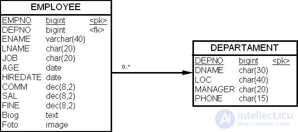
The "Employee" (EMPLOYEE) table is described in Example 20.1 of this lecture, and the description of the "Department" (DEPARTAMENT) table is given in Table 20.2 below.
| No. | Attribute name | Column name |
|---|---|---|
| 1 | Department number | DEPNO (PK) |
| 2 | Department name | DNAME |
| 3 | Location | LOC |
| 4 | Manager | MANAGER |
| 5 | Phone | PHONE |
Both tables are non-clustered and each is stored on its own physical pages. Suppose query analysis shows that in 80% of queries these two tables are used together, with the join performed on the "Department number" column (DEPNO). We could build a cluster for these two tables.
Before clustering, the tables are stored separately, each in its own physical area on disk.
| DEPARTAMENT | |||
| DEPNO | DNAME | LOC | …. |
| 10 | Trade | Moscow | |
| 20 | Consulting | Chernogolovka | |
| EMPLOYEE | |||
| EMPNO | ENAME | LNAME | DEPNO |
| 996 | Kozyrev | Sergey | 10 |
| 997 | Sapegin | Alexey | 20 |
After clustering on the "Department number" column (DEPNO), the rows of the tables will be stored together, sharing the same physical database pages.
| CLUSTER | ||||
| DEPNO | ||||
| 10 | DNAME | LOC | …. | |
| Trade | Moscow | …. | ||
| …. | …. | …. | ||
| EMPNO | ENAME | LNAME | …. | |
| 996 | Kozyrev | Sergey | …. | |
| …. | …. | …. | ||
| 20 | DNAME | LOC | …. | |
| Consulting | Chernogolovka | …. | ||
| EMPNO | ENAME | LNAME | …. | |
| 997 | Sapegin | Alexey | …. | |
| … | …. | …. | …. | |
The example shows that when joining the tables, the number of I/O operations required to access the cluster will be lower. It also shows that the value of the cluster key is stored only once in the cluster and/or the cluster index, regardless of how many rows from the different tables contain that value.
Clustering can substantially speed up join processing. However, when planning to use clusters, the following factors should be taken into account.
For the reasons listed above, clusters are not recommended for tables with heavy update activity. For a table to be a good candidate for clustering, at least the following conditions should hold:
It follows that there are two main reasons for using clusters: a) the need to provide direct access to a row in a single read operation, and b) the need to reduce the number of I/O operations when accessing data that is frequently used together, by placing it on physically nearby database pages.
From a physical standpoint, a cluster exists separately from the tables. It is created with specified storage parameters, and then clustered tables are created within it one after another. When describing a cluster, you need to specify the column or columns for which the DBMS will build the cluster, and the tables that will be included in it. When processing data, the DBMS places rows that contain the same values in the cluster columns as physically close together as possible. As a result, the rows of a table may be spread across several disk pages, but primary and foreign keys are usually placed on the same page.
Example 20.22.
Let's create a cluster for the "Department" (DEPARTAMENT) and "Employee" (EMPLOYEE) tables. Clusters are created using the SQL CREATE CLUSTER command, which in our case will look like this:
CREATE CLUSTER emp_dept_c (DEPNO integer)
SIZE 512,
-- TABLESPACE …
-- STORAGE …
INDEX;
CREATE TABLE DEPARTAMENT
   (
   DEPNO 	integer NOT NULL,
   DNAME 	char(20),
   LOC   		char(30),
   MANAGER  	char(20),
   PHONE  	char(15),
   CLUSTER emp_dept_c (DEPNO)
);

 CREATE TABLE EMPLOYEE
(
   EMPNO  	integer NOT NULL,
   ENAME  	char(40),
   LNAME  	char(20),
   DEPNO  	int NOT NULL,,
   JOB  		char(20),
   AGE  		date,
   HIREDATE  	date NOT NULL WITH DEFAULT,
   SAL  		dec(8,2),
   COMM  	dec(8,2),
   FINE  		dec(8,2),
   Biog 		text,
   Foto 		image,
   PRIMARY KEY (EMPNO),
   CLUSTER emp_dept_c (DEPNO)
);

CREATE INDEX emp_dept_c_id ON CLUSTER emp_dept_c;
The SIZE parameter defines the size of the cluster — in effect, the maximum number of cluster keys that can be stored on a single physical data page. The INDEX keyword means that the cluster being created is an index cluster.
The CLUSTER emp_dept_c (DEPNO) clause tells the DBMS that the table should be added to the cluster. Note that in the "Department" (DEPARTAMENT) table the primary key constraint on the "Department number" (DEPNO) column has been removed. This is because Oracle automatically creates an index on the primary key, and that index is not needed in this case. The last statement creates a cluster index for the cluster key of the cluster.
In one of the previous sections we already discussed the use of hash tables, which are in fact one way of implementing a cluster. Let's now look in detail at how to work with a hash cluster in Oracle.
Recall that hashing is a way of storing data tables in order to increase retrieval performance. The physical mechanism used to implement hashing in Oracle is the hash cluster. Data is retrieved from a hash cluster according to a hash function, which is used to map the distribution of the table's key values onto numeric values that determine physical database pages. A hash cluster is an alternative technique for building data tables, as opposed to an index cluster or a non-clustered table.
Example 20.23.
Let's take our sample database and create a hash cluster for the "Employee" (EMPLOYEE) table. The query for accessing the table's records before and after clustering is given below.
SELECT * FROM EMPLOYEE WHERE EMPNO= 997;
Before clustering on the "Employee number" (EPMNO) column, access is performed through an index, and, as shown in Fig. 20.9, it takes 4 I/O operations to obtain the resulting row.
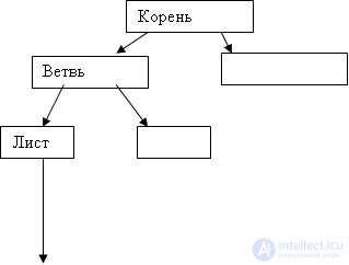
After clustering on the "Employee number" (EPMNO) column, the rows of the "Employee" (EMPLOYEE) table will be stored in a structure shown schematically in the figure below. After the key is hashed, it takes a single I/O operation to obtain the resulting row, provided there are no overflow chains.
| CLUSTER | ||||
| Hash key | Cluster key | |||
| 110 | EMPNO | ENAME | LNAME | …. |
| 996 | Kozyrev | Sergey | …. | |
| …. | …. | …. | ||
| 120 | EMPNO | ENAME | LNAME | …. |
| 997 | Sapegin | Alexey | …. | |
In a hash cluster, related rows (in this case, rows with the same hash key value) are likewise stored on the same physical database page, based on the hashed values of their shared key. In indexed tables and index clusters, on the other hand, the resulting row is located using key values stored in a separate index (see the CREATE INDEX example above for the cluster index).
Example 20.24.
Let's create a hash cluster for the "Employee" (EMPLOYEE) table from Example 20.21.
CREATE CLUSTER PERSONNEL (EMPNO integer)
SIZE 512
HASHKEYS 500
-- STORAGE (INITIAL 100K  NEXT 50K  PCTINCREASE 10)
;
The number of unique hash key values is set by the HASHKEYS parameter; once this value is reached, collisions will start occurring in the table — situations in which different hashed keys must be placed in the same block. This leads to the creation of so-called overflow chains when rows are inserted, and their presence increases the number of accesses needed to retrieve a resulting row.
The SIZE parameter defines the maximum number of hash keys placed on a physical database page. It equals the estimated total space in bytes required to store the average number of rows associated with each hash key value. If the available space on a page is 1600 bytes and the parameter value is 512 bytes, then three hash key values will be distributed across the physical page.
The HASH IS clause can be used to override the hash function that Oracle uses by default.
Example 20.25.
продолжение следует...
Часть 1 Designing data warehouse performance — indexing
Часть 2 Improving query performance: partitioning - Designing data warehouse performance —
Часть 3 Improving query performance: clusters - Designing data warehouse performance —
Часть 4 Summary - Designing data warehouse performance — indexing

Comments