
Lecture
Это продолжение увлекательной статьи про физическая модель хранилища данных.
...
font-family: "lucida grande", tahoma, verdana, arial, sans-serif; font-size: 12px;">
As noted above, the first step in building the physical model of a data warehouse is identifying the database tables. In solving this task, the data warehouse designer takes as input the relations of the logical data model that represent the entities of the domain, and as output of this modeling stage must produce definitions of the tables, their columns, keys, indexes, and so on.
Base tables are created for each relation of the logical model and are the primary data-storage objects in the database. For each base table, a long identifier is defined that uniquely identifies the table within the database. This name should conform to the naming standards for domain entities, if such standards were developed by the data administrator during the domain analysis stage.
For our teaching example, let's create five tables: four dimension tables — "Time", "Customer", "Product", "Employee" — and one fact table, "Sale". The table names will match the entity names of the data warehouse's logical model (fig. 11.3).
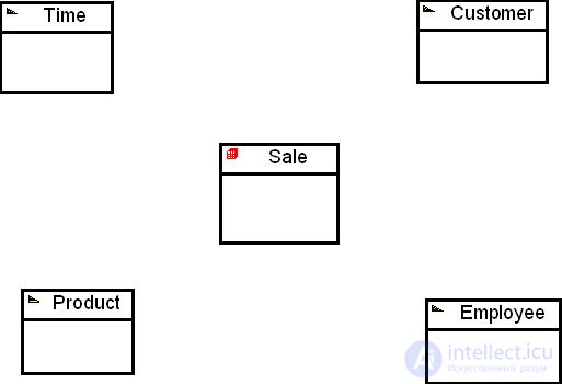
Once the designer has finished processing all the relations of the logical data model, they should double-check that the number of base tables matches the number of relations in the logical data model (i.e., no fewer than the number of entities in the domain). Thus, when creating base tables, the designer follows the principle: one base table per relation of the logical data model.
The next step for the data warehouse designer is identifying the columns for the base tables. Columns of a table should represent the attributes of the relations in the logical model of the relational data warehouse. These attributes must be converted into column specifications in the CREATE TABLE command. A column specification has the following syntax: column name, data type for the values stored in the column, and a list of constraints.
First, let's consider the task of adding columns. A column must have a name. The names of the attributes of the corresponding relations of the logical model are converted into column names according to the object-naming rules adopted in the specific DBMS. As noted above, this usually involves a restriction on name length and on the use of special characters in names. For example, some DBMSs allow a dollar sign in a name, but this character is often not recognized in data-retrieval commands – SELECT.
There is one more issue with naming columns – column names must be interpreted unambiguously by users. For example, if the designer assigns the short name LN to an employee's last name, a comment will probably be needed to clarify that this stands for last name and not, say, a production line. If for some reason long field names cannot be used, a data dictionary should be used to interpret the abbreviations introduced.
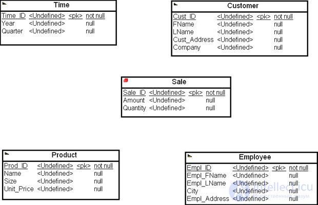
For our teaching example, solving this task comes down to transferring the entities' attributes into the fields of the corresponding database tables. Note that attributes that are candidates for foreign keys are not carried over. Fig. 11.4 shows the result of this work.
Note that to maintain the principle of field-name uniqueness within the model when defining fields based on entity attribute names, we changed some names. For instance, the "Address" attribute of the "Employee" entity became "Employee address" (Empl_Address) in the corresponding "Employee" table of the physical model. Likewise, the "Address" attribute of the "Customer" entity became "Customer address" (Cust_Address) in the corresponding "Customer" table of the physical model.
After identifying the columns, their type must be set according to the data types supported by the given DBMS. This task is simplified if attribute domains have been defined in the relations of the logical model. Some domains may already be defined in terms of the DBMS. For such attributes, virtually nothing needs to be done: the domain definition in terms of the DBMS data type just needs to be carried over into the column specification. The designer may need to refine minor type parameters. For example, if a domain is specified as DEC(9,2), but the domain context indicates that this column will accumulate a running total of annual expenses, it may be advisable to define the type as DEC(15,2) to avoid possible overflow when the database applications run.
If a domain is not defined in terms of the DBMS, the database designer must convert it into a suitable data type. When performing such conversions, a number of factors should be taken into account.
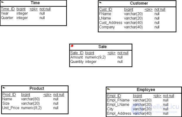
In our teaching example, a domain has been defined for every attribute. For the entities' surrogate primary identifiers, this is a numeric value. Given that the data warehouse will store large volumes of data, it makes sense to use the bigint data type to represent such attributes in the database, and the integer data type for the remaining attributes. The "Text" domain can be represented with the varchar(n) data type, and for representing decimal numbers, the numeric (p, s ) data type can be used.
The result of determining the column types for the data warehouse's physical model tables is shown in fig. 11.5.
After defining all the columns and their types, the next step is identifying the primary keys of the tables. According to the requirements of relational theory, every row (tuple) of a table must have a unique primary key. Usually, a good candidate for a table's primary key is the primary key of the corresponding relation in the logical model. Since the logical-model relation is assumed to already have a primary key possessing the property of minimality, it simply needs to be declared in the CREATE TABLE command. For many tables, this definition of the primary key is not final. The primary key may be redefined at later stages of physical database design.
In many DBMSs, including the MS SQL Server family, designating a column as a primary key is treated as a constraint on the column's value (see later in this lecture).
For our example, we have already defined the primary keys of the data warehouse's physical model tables as the primary keys of the corresponding entities.
After completing the steps above, the task of defining the primary keys of the base tables can be considered done as a first approximation, and we can move on to the next important table-definition task – defining constraints on column values.
When defining table column specifications, the designer must consider the constraints that can be imposed on column values. Relational DBMSs support quite a few such constraints. Here we will focus on one of the main ones – the requirement that a column always have a value. This constraint on a column's values is called a NOT NULL constraint.
A predefined column value of NULL means that, at a given moment, for a given row (an instance of a domain entity), the value is undefined, unknown, or absent. The database designer must identify whether a column can take NULL values, since users may run into problems when working with such columns.
One example of such a problem is a situation where a user needs to join two tables on columns that contain NULL values. When performing joins, any rows that have NULL values in the join columns in either table will not appear in the resulting query output. Such data loss can cause the user to get an incorrect result set for the query, especially if they need to see all rows from at least one of the tables.
When assigning NULL values to columns, the designer needs to take the following factors into account.
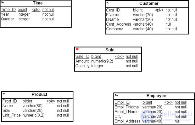
For our teaching example, all columns of the data warehouse's physical model tables, perhaps with the exception of addresses, should have a NOT NULL constraint (fig. 11.6).
The next step in modeling the physical model of the data warehouse is establishing relationships between the tables of the data warehouse model.
The dimension tables and the fact table in a multidimensional data model are in a "parent-child" relationship. The primary key and its corresponding foreign key implement the parent/child relationship between tables of a relational database. They reflect the relationship between objects of the domain (represented by table tuples) through the values of some of their attributes, following the principle of hierarchical subordination, whereby the parent object determines the existence of child objects. The child objects themselves may also act as parents for other objects (descendants).
A relational database table that contains the primary key is called the parent table, while the table containing the foreign key corresponding to that primary key is called the child table. In our teaching example, the "Product" dimension table is the parent table for the "Sale" fact table.
The "parent-child" relationship between tables is implemented through the key attributes of the corresponding rows. A row belonging to the parent table is called a parent row, while a row in the child table that is referenced by the parent row is called a child row. A child row must have at least one non-null foreign-key attribute.
The "parent-child" relationships between two tables reflect an inclusion relationship on the domains of the corresponding attributes.
Having established the "parent-child" relationship between the dimension tables and the fact table in our teaching example, we obtain the physical model of the data warehouse (fig. 11.7)
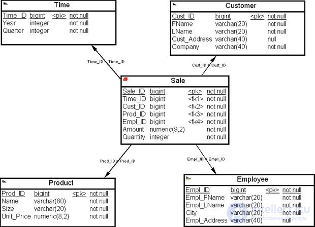
A question that needs to be resolved when modeling the data warehouse is whether the dimensions' foreign keys should be elements of the fact table's composite primary key.
In our example, the fact table has a unique surrogate key, "Sale identifier" ( Sale_ID ), so the foreign keys implementing the "parent-child" relationship between the dimension tables and the fact table do not necessarily need to be included in the fact table's composite primary key. Any row of the fact table is already uniquely identified by the assigned primary key.
After creating the physical model of the data warehouse, the designer can move on to the task of developing the script to create the data warehouse. This task can be solved either manually, as we will do in the next section of this lecture, or with the help of CASE tools.
SQL provides the CREATE TABLE command for defining and creating tables, which specifies the table name, the names and physical order of its columns, the type of each column, as well as various instructions for the DBMS, such as defining a primary or foreign key, requirements prohibiting undefined values in a table column, and so on.
The CREATE TABLE command creates a new table in the database. The syntax of this command for the SQL dialect (Transact-SQL) of the MS SQL Server family of DBMSs is given below.
CREATE TABLE
    [ database_name . [ schema_name ] . | schema_name . ] table_name
        ( {  |
                |  }
        [  ] [ ,...n ] )
    [ ON { partition_scheme_name ( partition_column_name ) | filegroup
        | "default" } ]

    [ { TEXTIMAGE_ON { filegroup | "default" } ]
    [ FILESTREAM_ON { partition_scheme_name | filegroup
        | "default" } ]
    [ WITH (  [ ,...n ] ) ]
[ ; ]

 ::=
column_name
    [ FILESTREAM ]
    [ COLLATE collation_name ]
    [ NULL | NOT NULL ]
    [
        [ CONSTRAINT constraint_name ] DEFAULT constant_expression ]
      | [ IDENTITY [ ( seed ,increment ) ] [ NOT FOR REPLICATION ]
    ]
    [ ROWGUIDCOL ] [  [ ...n ] ]
    [ SPARSE ]

 ::=
[ type_schema_name . ] type_name
    [ ( precision [ , scale ] | max |
        [ { CONTENT | DOCUMENT } ] xml_schema_collection ) ]

 ::=
[ CONSTRAINT constraint_name ]
{     { PRIMARY KEY | UNIQUE }
        [ CLUSTERED | NONCLUSTERED ]
        [
            WITH FILLFACTOR = fillfactor
          | WITH ( < index_option > [ , ...n ] )
        ]
        [ ON { partition_scheme_name ( partition_column_name )
            | filegroup | "default" } ]
  | [ FOREIGN KEY ]
        REFERENCES [ schema_name . ] referenced_table_name [ ( ref_column ) ]
        [ ON DELETE { NO ACTION | CASCADE | SET NULL | SET DEFAULT } ]
        [ ON UPDATE { NO ACTION | CASCADE | SET NULL | SET DEFAULT } ]
        [ NOT FOR REPLICATION ]
  | CHECK [ NOT FOR REPLICATION ] ( logical_expression )
}
 ::=
column_name AS computed_column_expression
[ PERSISTED [ NOT NULL ] ]
[
    [ CONSTRAINT constraint_name ]
    { PRIMARY KEY | UNIQUE }
        [ CLUSTERED | NONCLUSTERED ]
        [
            WITH FILLFACTOR = fillfactor
          | WITH (  [ , ...n ] )
        ]
    | [ FOREIGN KEY ]
        REFERENCES referenced_table_name [ ( ref_column ) ]
        [ ON DELETE { NO ACTION | CASCADE } ]
        [ ON UPDATE { NO ACTION } ]
        [ NOT FOR REPLICATION ]
    | CHECK [ NOT FOR REPLICATION ] ( logical_expression )
    [ ON { partition_scheme_name ( partition_column_name )
        | filegroup | "default" } ]
]

 ::=
column_set_name XML COLUMN_SET FOR ALL_SPARSE_COLUMNS

< table_constraint > ::=
[ CONSTRAINT constraint_name ]
{
    { PRIMARY KEY | UNIQUE }
        [ CLUSTERED | NONCLUSTERED ]
                (column [ ASC | DESC ] [ ,...n ] )
        [
            WITH FILLFACTOR = fillfactor
           |WITH (  [ , ...n ] )
        ]
        [ ON { partition_scheme_name (partition_column_name)
            | filegroup | "default" } ]
    | FOREIGN KEY
                ( column [ ,...n ] )
        REFERENCES referenced_table_name [ ( ref_column [ ,...n ] ) ]
        [ ON DELETE { NO ACTION | CASCADE | SET NULL | SET DEFAULT } ]
        [ ON UPDATE { NO ACTION | CASCADE | SET NULL | SET DEFAULT } ]
        [ NOT FOR REPLICATION ]
    | CHECK [ NOT FOR REPLICATION ] ( logical_expression )
}

 ::=
{
    DATA_COMPRESSION = { NONE | ROW | PAGE }
      [ ON PARTITIONS ( {  |  }
            [ , ...n ] ) ]
}

 ::=
{
    PAD_INDEX = { ON | OFF }
  | FILLFACTOR = fillfactor
  | IGNORE_DUP_KEY = { ON | OFF }
  | STATISTICS_NORECOMPUTE = { ON | OFF }
  | ALLOW_ROW_LOCKS = { ON | OFF}
  | ALLOW_PAGE_LOCKS ={ ON | OFF}
  | DATA_COMPRESSION = { NONE | ROW | PAGE }
       [ ON PARTITIONS ( {  |  }
       [ , ...n ] ) ]
}
 ::=
 TO
Let's look at the elements and arguments of the CREATE TАBLE command.
Computed columns can be used in select lists, WHERE clauses, ORDER BY clauses, and anywhere else that ordinary expressions can be used, with the following exceptions.
The ON {
The TEXTIMAGE_ON parameter is not allowed if the table has no large-value columns. The TEXTIMAGE_ON parameter cannot be specified together with the
If a table contains FILESTREAM data and is partitioned, the FILESTREAM_ON clause must be included, specifying the filegroup partition scheme for the FILESTREAM data. This partition scheme must use the same partitioning functions and columns as the partition scheme used for the table; otherwise an error occurs.
If the table is not partitioned, the FILESTREAM column cannot be partitioned either. FILESTREAM data for the table must be stored in a separate filegroup. This filegroup is specified in the FILESTREAM_ON clause.
If the table is not partitioned and the FILESTREAM_ON clause is not specified, the FILESTREAM filegroup marked with the DEFAULT property is used. If there is no FILESTREAM filegroup, an error occurs.
As with the ON and TEXTIMAGE_ON clauses, the value specified with the CREATE TABLE statement for the FILESTREAM_ON clause cannot be changed, except in the following situations.
The data type can be one of the following.
 bytes of character and binary data, or 2^30 bytes of Unicode data.
продолжение следует...
Часть 1 The physical model of a data warehouse
Часть 2 Developing a script for creating the objects of the data
Часть 3 Constraints and their use in a relational database - The
Часть 4 Summary - The physical model of a data warehouse

Comments