Column denormalization - The physical model of a data warehouse:

Это окончание невероятной информации про хранилища данных и учет влияния транзакций.

...

whole.

The frequency of field usage in transactions is given in table 19.1.

Table 19.1 does not contain the frequency of joint use of columns in transactions, but from the frequencies of field usage in transactions one can draw a conclusion about the joint use of columns. It is most likely that columns with similar usage frequency values are also used together.

Thus, there is a basis for deciding to split the "Employees" (EMPLOYEE) table into two — say, "Employees" (EMPLOYEE_BASE) and "Additional data" (ADD_EMPL), as shown in fig. 19.7.

Fig. 19.7. Vertical partitioning of the "Employees" (EMPLOYEE) table into two tables: "Employees" (EMPLOYEE_BASE) and "Additional data" (ADD_EMPL)

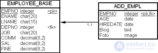
The sequence of SQL commands for creating the vertical partitioning of the "Employees" table is given below.

create table ADD_EMPL (
   EMPNO             integer           not null,
   AGE                  date                null,
   HIREDATE       date               not null with default,
   Biog                 text                  null,
   Foto                 image              null,
   constraint PK_ADD_EMPL primary key (EMPNO)
)
go

create table EMPLOYEE_BASE (
   EMPNO                integer              not null,
   ENAME                char(20)             null,
   LNAME                char(15)             null,
   DEPNO                integer              null,
   JOB                      char(20)             null,
   COMM                 decimal(8,2)         null,
   SAL                      decimal(8,2)         null,
   FINE                     decimal(8,2)         null,
   constraint PK_EMPLOYEE_BASE primary key (EMPNO)
)
go

alter table ADD_EMPL
   add constraint FK_ADD_EMPL_REFERENCE_EMPLOYEE foreign key (EMPNO)
      references EMPLOYEE_BASE (EMPNO)
go

alter table EMPLOYEE_BASE
   add constraint FK_EMPLOYEE_REFERENCE_DEPARTAMENT (DEPNO)
      references DEPARTAMENT (DEPNO)
go

We defined the referential integrity constraint between the "Employees" (EMPLOYEE_BASE) and "Additional data" (ADD_EMPL) tables using the ALTER TABLE command, so it will be maintained by the built-in mechanisms of the MS SQL Server 2008 DBMS.

In addition to improving the performance of retrieval operations, another justification for vertical table partitioning is improved performance for insert and delete operations, as well as for backup and recovery operations for the DB or data warehouse.

Long rows in hash tables

Many relational DBMSs support so-called clustered hash indexes (clustered hashed index). Such objects are more correctly called hash tables rather than indexes. A hash table is a relational database table in which access to rows is performed via a key transformation. The values of the columns declared as key columns are transformed into row positions in the table (and are placed there when inserted) – that is, they are hashed. Such a function is called a hash function. The table key subjected to the transformation is called the hash key.

Data processed in this way are placed in special tables, also called hash clusters or simply hash tables. In this lecture, we assume that the designer already knows the general methods of organizing physical data access, so we will not discuss in detail how such tables are structured.

Note that hashing is a very efficient method of accessing a record by primary key in a single access. If the key values are uniformly distributed, this will hold on average. Otherwise, access performance will drop sharply due to collisions — cases where the hash function produces the same number, i.e. the same record position, for two different primary key values. In the worst case, the entire table will have to be scanned to obtain a single record.

Although dynamic hash tables have been built (which change their size over their lifetime), most DBMSs support static hash tables, whose size is determined at creation time. In most cases, a hash table is organized in a manner that is essentially random with respect to the order of key values, although key transformation functions are known that preserve a lexicographic order on the table's key values.

A hash index is usually used when the key is fully represented in the WHERE clause and an equality operation is used for the key columns.

We are interested in the problem of increasing performance in hash tables when the row length exceeds the size of a physical page on disk. To better understand the problem, let us look at how a hash table is defined in SQL.

Such a table is created using a command such as (as in the SQLBase DBMS):

CREATE CLUSTERED HASHES INDEX CHXNAME ON EMPLOYEE
(EMPNO) SIZE 2000 ROWS;

The SIZE clause specifies the estimated number of rows in the index, and ROWS defines the number of rows for storing the index. The size can also be specified in blocks (BUCKETS). Thus, the primary key value is used to address a block containing an integer number of rows, or a single row if its size is comparable to the size of the physical block. In the latter case, the block is considered to contain one row.

For a hash table, a parameter called "rows per page", or page clustering, or the blocking factor, is defined, equal to

As can be seen from the definition of a hash table, the row size and the physical block size must be consistent. The problem of a long row in a hash table is that if a row occupies several blocks, the frequency of collisions increases, and instead of a single physical access to retrieve a row, 4-6 accesses are required, which is already comparable to using an index of a different type.

The goal of partitioning a hash table is to try to achieve a value of the blocking factor (blocking factor) at which the table would contain as many rows as possible that are retrieved together in most transactions against this table.

Since in modern DBMSs the size of a physical block is fixed for each operating platform, the only way to influence this parameter is by adjusting the row size. If it is not possible to revise the specification of the table's column types and reduce their sizes to a minimum, the only way to choose a suitable blocking factor is to partition the hash table.

In the MS SQL Server family of DBMSs, hash tables are not explicitly supported. However, they can be created using the CHECKSUM() function together with a computed column in an index. The index must be non-unique so that hash function collisions can be resolved.

Horizontal partitioning of tables

In practice, horizontal partitioning (horizontally partition) is used to isolate one group of table rows from another when the use of these groups of rows in transactions almost never overlaps. A typical example is the isolation of current data from archived data.

Consider an order processing system. Managers and salespeople work with current orders. Processing of completed orders (archived data) is performed when preparing various kinds of reports (in particular, by creating a data mart). Even if a daily report is prepared that accesses archived data, in mid-sized organizations the frequency of use of current data still exceeds the frequency of use of archived data by 2-3 orders of magnitude, and the ratio of the volume of current data to archived data can be less than 0.001.

One of the practical criteria in this case can be the classic 80-20 rule. If 20 percent of the data is actively worked with, then most likely the remaining 80% can be moved to an archive table.

Example 19.6.

A table that is a candidate for horizontal partitioning is the "Project" (PROJECT) table, whose structure is shown in fig. 19.8. This table stores archived data – completed projects.

Fig. 19.8. "Project" table (PROJECT)

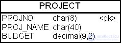
Suppose that the number of completed projects per year in the organization is around 1000. The data needs to be kept in the tables for 10 years (10,000 records). The average project duration is two months, i.e., the number of unfinished projects at any given time does not exceed 200. After 5 years, the ratio of the number of current projects to archived projects will reach 0.04.

Consequently, it is worth considering horizontal partitioning of this table and carrying it out as shown in fig. 19.9.

Fig. 19.9. Horizontal partitioning of the "Project" (PROJECT) table into two tables: "Current projects" (PROJECT_CUR) and "Archived projects" (PROJECT_OLD)

We split the "Project" (PROJECT) table horizontally into two tables — "Current projects" (PROJECT_CUR) and "Archived projects" (PROJECT_OLD). The sequence of commands for creating the partitioned tables is given below.

create table PROJECT_CUR (
   PROJNO               char(8)              not null,
   PROJ_NAME            char(40)             not null,
   BUDGET               decimal(9,2)         not null,
   constraint PK_PROJECT_CUR primary key (PROJNO)
)
go

create table PROJECT_OLD (
   PROJNO               char(8)              not null,
   PROJ_NAME            char(40)             not null,
   BUDGET               decimal(9,2)         not null,
   constraint PK_PROJECT_OLD primary key (PROJNO)
)
go

For joint use of these two tables, a view "All projects" (ALL_PROJECT) can be provided, which is shown in fig. 19.10.

Fig. 19.10. The "All projects" view (ALL_PROJECT)

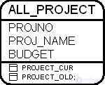
The SQL command for creating the "All projects" view (ALL_PROJECT) is given below.

CREATE VIEW ALL_PROJECT
AS
SELECT PROJNO, PROJ_NAME, BUDGET FROM PROJECT_CUR
UNION
SELECT PROJNO, PROJ_NAME, BUDGET FROM PROJECT_OLD;

Note that hereafter, the term "original table" refers both to the table itself and to what it became after partitioning.

Table partitioning and referential integrity

If the table was normalized before partitioning, the primary keys will be identical for the tables resulting from the partitioning. Consequently, the relationships of the new tables with other tables in the database may remain the same as with the original table. However, it is also necessary to consider the delete rules for the original table, and the participation of the new table in existing referential integrity relationships, when deciding how to support referential integrity in the new tables.

In some cases, it may be simpler not to define referential integrity at all, since actual deletion of rows from the new table will be maintained in parallel with the original table by some programmatic means in the database application (for example, using a trigger).

Example 19.7.

To resolve the many-to-many relationship between the "Employee" (EMPLOYEE) and "Project" (PROJECT) tables, a linking table "Employee Project" (EMP_PROJ) was introduced, which has referential integrity constraints with the "Project" (PROJECT) table, as shown in fig. 19.11.

Fig. 19.11. Resolving the many-to-many relationship between the "Employee" (EMPLOYEE) and "Project" (PROJECT) tables

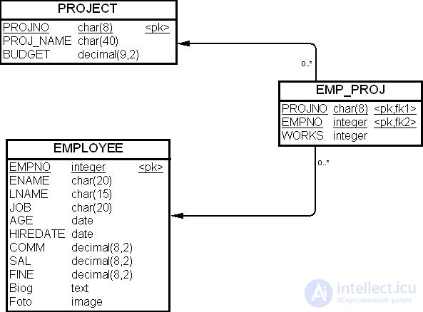
The linking table "Employee Project" (EMP_PROJ) was created using the SQL command given below.

create table EMP_PROJ (
   PROJNO               char(8)              not null,
   EMPNO                integer              not null,
   WORKS                integer              null,
   constraint PK_EMP_PROJ primary key (PROJNO, EMPNO).
   constraint FK_EMP_PROJ_REFERENCE_PROJECT foreign key (PROJNO)
      references PROJECT (PROJNO),
   constraint FK_EMP_PROJ_REFERENCE_EMPLOYEE foreign key (EMPNO)
      references EMPLOYEE (EMPNO)
)
go

But now, after partitioning the "Project" (PROJECT) table, we have two new tables: "Current projects" (PROJECT_CUR) instead of the "Projects" (PROJECT) table, and "Archived projects" (PROJECT_OLD), as shown in fig. 19.12.

Fig. 19.12. Resolving the many-to-many relationship after partitioning the "Projects" (PROJECT) table

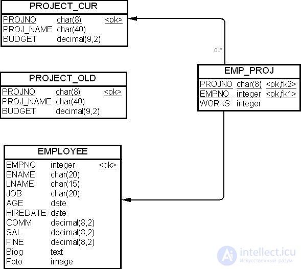
Suppose that to carry out a project the organization hires employees on a temporary basis (for the duration of the project), and management is not interested in the question of who did which projects and when. In this case, management is not interested in the relationship between performers and projects that have already been completed, and consequently, nothing needs to be changed in the physical data model.

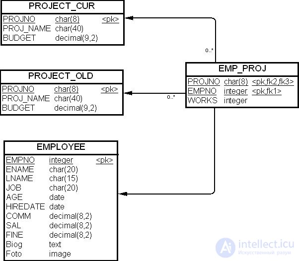
However, if the relationship between performers and completed projects must be tracked (for example, management wants to investigate who performed which project and when), it should also be extended to the "Archived projects" (PROJECT_OLD) table, as shown in fig. 19.13.

To reflect the work we have done in the database, it is enough to add a foreign key constraint to the "Employee Project" (EMP_PROJ) table, as shown below:

Fig. 19.13. Resolving the many-to-many relationship for the "Archived projects" (PROJECT_OLD) table

drop table EMP_PROJ
Go

create table EMP_PROJ (
   PROJNO               char(8)              not null,
   EMPNO                integer              not null,
   WORKS                integer              null,
   constraint PK_EMP_PROJ primary key (PROJNO, EMPNO).
   constraint FK_EMP_PROJ_REFERENCE_PROJECT foreign key (PROJNO)
      references PROJECT_CUR (PROJNO),
   constraint FK_EMP_PROJ_REFERENCE_PROJECT_OLD foreign key (PROJNO)
      references PROJECT_OLD (PROJNO),
   constraint FK_EMP_PROJ_REFERENCE_EMPLOYEE foreign key (EMPNO)
      references EMPLOYEE (EMPNO)
)
go

When partitioning a table for which referential integrity constraints have been defined, one can also consider supporting referential integrity by establishing a "one-to-one" relationship pointing from the new table back to the original table. In this case, the new table will have a foreign key identical to the table's primary key. For example, a "one-to-one" relationship between the tables in fig. 19.14.

Fig. 19.14. A "one-to-one" relationship between the "Current projects" (PROJECT_CUR) and "Archived projects" (PROJECT_OLD) tables

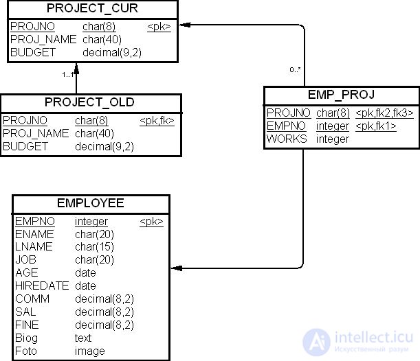
If a cascading delete rule is defined for this foreign key (see "Introduction to the CASE tool"), the DBMS will automatically delete rows of the new table when the corresponding row of the original table is deleted, although insertion of rows will have to be managed at the application level for the data warehouse. The SQL command for this case is given below.

create table PROJECT_OLD (
   PROJNO               char(8)              not null,
   PROJ_NAME            char(40)             not null,
   BUDGET               decimal(9,2)         not null,
   constraint PK_PROJECT_OLD primary key (PROJNO),
   constraint FK_EMP_PROJ_REFERENCE_PROJECT_OLD_1 foreign key (PROJNO)
      references PROJECT_СUR (PROJNO)
)
go

When deciding to partition a table, the following algorithm should be followed:

• determine which columns of the original table will be moved into which new tables;
• create the new tables with a primary key identical to the primary key of the original table;
• if the DBMS is to manage declarative referential integrity for the new tables in the same way as for the original table, in the case where it is a child table in a relationship, a foreign key column referencing each parent table in the relationship should be added to the new table, i.e., the new table should contain a foreign key constraint identical to that of the parent table for each relationship. An alternative to this solution is to create a "one-to-one" relationship between the new table and the original table, defining a foreign key back to the original table identical to the primary key;
• if the DBMS is to manage referential integrity for the new tables in the same way as for the original table, in the case where it is the parent table in a relationship, a foreign key should be added to each child table of the original table to identify the new table as the parent. One can also proceed as in the first part of the previous point, in which case the new tables should not be declared as parents in other relationships. The original table maintains all relationships in which it acts as the parent;
• application developers should be given all the INSERT commands for the tables resulting from partitioning, or given the rules that row insertion into these tables must follow;
• all views based on the original table should be modified, and, if needed, the creation of new views for accessing the new tables should be considered.

Merging database tables

Table collapsing is the process of moving rows from several tables into one new table in order to limit the number of database table joins and improve query performance.

The merged table includes the columns of all the tables being merged. If referential integrity constraints were established between the tables, then during the merge the parent table's columns are duplicated, the foreign key constraints of the child tables are removed from the merged table, and the columns used for joining the merged tables are removed.

Let's consider some examples.

Example. 13.8.

Suppose it was decided to merge the "Customer" and "Order" tables — they need to be merged in order to eliminate the join operation in queries against these tables. The physical data model before the merge is shown in fig. 19.15.

enlarge image
Fig. 19.15. The "Customer" and "Order" tables before their merge

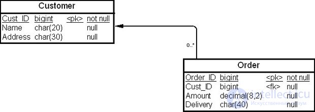
As a result of merging the tables, a single table "Customer Order" (Cust_Order) will be created, containing all the columns of the merged tables (fig. 19.16).

Fig. 19.16. The "Customer Order" (Cust_Order) table, merging the "Customer" and "Order" tables

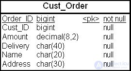
The SQL command for creating the merged table is given below.

create table Cust_Order (
   Order_ID             bigint               not null,
   Cust_ID              bigint               not null,
   Amount               decimal(8,2)         null,
   Delivery             char(40)             null,
   Name                 char(20)             null,
   Address              char(30)             null,
   constraint PK_CUST_ORDER primary key (Order_ID)
)
go

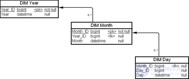
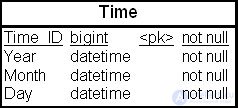
For a data warehouse, it is worth considering merging normalized hierarchy tables — for example, dimension tables representing the "Time" dimension (Time), as in fig. 19.17. A denormalized dimension table for the "Time" hierarchy is shown in fig. 19.18.

enlarge image
Fig. 19.17. Hierarchy of tables for the "Time" dimension

Fig. 19.18. Denormalized table for the "Time" hierarchy

Column denormalization

Column denormalization (Column denormalization) is a process for limiting the number of frequently occurring database table joins and improving query performance.

Let's consider the following example.

Example 19.9.

Let a physical data model be given (fig. 19.19).

Fig. 19.19. Tables of the physical data model

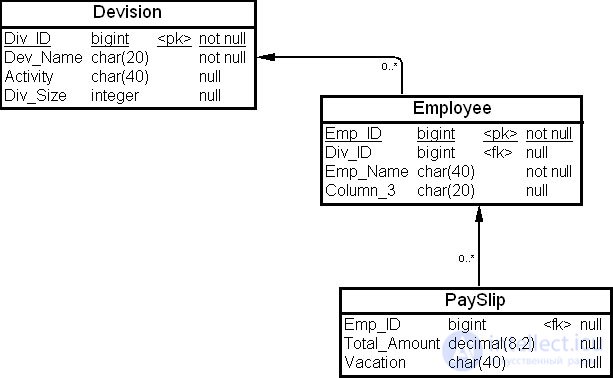
Suppose that a report needs to print the "Division name" (Div_name) column on the pay slip from the "Pay Slip" table for each employee. To solve this problem, one can consider denormalizing the table's columns so as to have the "Division name" (Div_Name) column in the "Pay Slip" table. For this, let's move the "Division name" (Div_Name) column (downward denormalization) into the "Pay Slip" table. The physical data model of the "Pay Slip" table is shown in fig. 19.20.

Fig. 19.20. Downward denormalization of the "Pay Slip" table

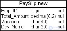
In this way, we reduce the number of joins when the "Pay Slip" table columns and the "Division Name" (Div_Name) column are used together in reports.

Summary

In this lecture we examined the process of denormalizing physical database tables at the physical data model design level, both for OLTP databases and for data warehouses.

Denormalization is a set of techniques for tuning the physical database model used to implement a data warehouse in order to meet its performance requirements. These techniques amount to a set of recommendations and heuristic rules for modifying the physical database structure obtained after the first iteration of building the physical data model of the data warehouse. Applying these techniques is advisory rather than mandatory.

This lecture described the various types of denormalization and the methods for implementing it. It also covered how to ensure data integrity during denormalization without resorting to additional code.

Thus, denormalization refers to the process of striking trade-offs in normalized tables by deliberately introducing redundancy in order to improve performance.

In most cases, the need for denormalization becomes apparent only at the stage of designing or operating the data warehouse application. In other words, a decision about denormalization cannot be made on the basis of the data model alone. Typically, one tries to identify the critical processes in the data warehouse's applications and makes denormalization decisions primarily in favor of these processes. Critical processes are generally identified by high frequency, large volume, high volatility, or explicit priority. A thorough description of database transactions makes it possible to identify the presence of such critical processes.

Продолжение:

Часть 1 The physical model of a data warehouse: accounting for the impact of transactions, table denormalization
Часть 2 Column denormalization - The physical model of a data warehouse: