Lecture
Stages of database development
The purpose of the development of any database is the storage and use of information about any subject area. To achieve this goal, the following tools are available:
However, it is obvious that for the same subject domain, relational relationships can be designed in many different ways. For example, you can design multiple relationships with a large number of attributes, or vice versa, spread all attributes across a large number of small relationships. How to determine on what grounds you need to put the attributes in certain relationships?
This chapter discusses the ways of "good" or "correct" design of relational relations. We will first discuss what "good" or "correct" data models mean. Then the concepts of the first, second and third normal forms of relations (1NF, 2NF, 3NF) will be introduced and it is shown that the relations in the third normal form are “good”.
When developing a database, several modeling levels are usually distinguished, with the help of which the transition from the subject area to a specific database implementation by means of a specific DBMS occurs. The following levels can be distinguished:
The subject area is a part of the real world, the data about which we want to be reflected in the database. For example, you can choose an enterprise accounting department, personnel department, bank, shop, etc. as a subject area. The subject area is infinite and contains both essential concepts and data, as well as little or no meaningful data. So, if you choose to take stock of goods in the warehouse as the subject area, then the concepts of "consignment note" and "invoice" are essential concepts, and the fact that an employee who accepts invoices has two children is not important for accounting of goods. However, from the point of view of the personnel department, data on the presence of children are essential. Thus, the importance of data depends on the choice of subject area.
Domain Model The domain model is our knowledge of the domain. Knowledge can be either in the form of informal knowledge in the brain of an expert, or expressed formally by any means. Such means may include textual descriptions of the subject area, sets of job descriptions, rules for conducting business in a company, etc. Experience shows that the text way of presenting a domain model is extremely inefficient. Much more informative and useful in the development of databases are descriptions of the subject area, made using specialized graphic notations. There are a large number of techniques for describing the subject area. Among the most well-known, we can call the SADT structural analysis method and IDEF0 based on it, Gein-Sarson data flow diagrams, the UML object-oriented analysis methodology, etc. The domain model describes more likely the processes that take place in the data domain and the data used by these processes. The success of further application development depends on how correctly the subject area is modeled.
Logical data model At the next lower level is the logical data model of the subject area. The logical model describes the concepts of the subject area, their relationship, as well as restrictions on the data imposed by the subject area. Examples of concepts - "employee", "department", "project", "salary". Examples of interrelationships between concepts - “an employee is listed in exactly one department”, “an employee can carry out several projects”, “several employees can work on one project”. Examples of restrictions - "employee age not less than 16 and not more than 60 years."
The logical data model is the initial prototype of the future database. The logical model is built in terms of information units, but without reference to a specific DBMS . Moreover, the logical data model does not necessarily have to be expressed by the means of the relational data model. The main means of developing a logical data model at the moment are various variants of ER-diagrams ( Entity-Relationship , entity-relationship diagrams ). The same ER model can be converted into a relational data model as well as a data model for hierarchical and networked DBMSs, or into a post-relational data model. However, since If we consider relational DBMS, then we can assume that the logical data model for us is formulated in terms of the relational data model.
Decisions made at the previous level, when developing a domain model, define some bounds within which a logical data model can be developed, and within these bounds, various decisions can be made. For example, the inventory domain model contains the concepts of “warehouse”, “invoice”, “product”. When developing an appropriate relational model, these terms must be used, but there are many different ways of implementation - you can create one relation in which the “warehouse”, “consignment note”, “goods” will be present, and you can create three separate relationships one for each concept.
When developing a logical data model, the following questions arise: are relationships well designed? Do they correctly reflect the domain model and, therefore, the domain itself?
Physical data model . At a lower level is the physical data model. The physical data model describes the data by means of a specific DBMS. We will assume that the physical data model is implemented by means of a relational DBMS, although, as mentioned above, this is not necessary. Relations developed at the stage of forming a logical data model are converted into tables, attributes become table columns, unique indexes are created for key attributes, domains are converted to data types accepted in a specific DBMS.
Constraints in the logical data model are implemented by various DBMS tools, for example, using indexes, declarative integrity constraints, triggers, and stored procedures. At the same time, again, decisions made at the level of logical modeling define some boundaries within which a physical data model can be developed. Similarly, various decisions can be made within these limits. For example, the relationships contained in the logical data model should be converted into tables, but for each table you can additionally declare different indexes that increase the speed of access to the data. Much depends on the specific DBMS.
When developing a physical data model, the following questions arise: are the tables well designed? Are the indexes correct? How much software code in the form of triggers and stored procedures need to be developed to maintain data integrity?
Actually database and applications . And finally, as a result of the previous steps, the database itself appears. The database is implemented on a specific software and hardware basis, and the choice of this basis allows you to significantly increase the speed of work with the database. For example, you can choose different types of computers, change the number of processors, RAM, disk subsystems, etc. Setting up the DBMS within the selected software and hardware platform is also very important.
But again, the decisions made at the previous level - the level of physical design, define the boundaries within which you can make decisions on the choice of software and hardware platform and DBMS settings.
Thus, it is clear that decisions made at each stage of modeling and database development will affect further steps. Therefore, making the right decisions at the early stages of modeling plays a special role.
Criteria for assessing the quality of a logical data model
The purpose of this chapter is to describe some principles for building good logical data models . Good in the sense that decisions made during the logical design process would lead to good physical models and ultimately good database performance.
In order to assess the quality of decisions made at the level of a logical data model, it is necessary to formulate some quality criteria in terms of a physical model and a specific implementation and see how the various decisions made during the logical modeling process affect the quality of the physical model and the speed of the database.
Of course, there may be a lot of such criteria and their choice is sufficiently arbitrary. We will consider some of these criteria, which are certainly important in terms of obtaining a high-quality database:
Adequacy of the domain database
The database should adequately reflect the subject area. This means that the following conditions must be met:
Ease of database development and maintenance
Virtually any database, with the exception of the completely elementary, contains a certain amount of program code in the form of triggers and stored procedures.
Stored procedures are procedures and functions that are stored directly in the database in compiled form and that can be run by users or applications that work with the database. Stored procedures are usually written either in a special procedural extension of the SQL language (for example, PL / SQL for ORACLE or Transact-SQL for MS SQL Server), or in some universal programming language, for example, C ++, with the inclusion of SQL statements in the code in accordance with special rules for such inclusion. The main purpose of stored procedures is the implementation of business processes in the subject area.
Triggers are stored procedures associated with some events that occur during database operation. These events are inserts, updates and deletes rows of tables. If a certain trigger is defined in the database, it will automatically start whenever an event occurs with which this trigger is associated. Very important is that the user can not bypass the trigger. A trigger is triggered regardless of which user or method triggered the event that triggered the trigger. Thus, the main purpose of triggers is to automatically maintain the integrity of the database. Triggers can be either quite simple, for example, supporting referential integrity, or quite complex, implementing any complex domain restrictions or complex actions that must occur when certain events occur. For example, a trigger may be associated with the operation of inserting a new product into an invoice; it performs the following actions — checks whether there is a necessary quantity of goods, adds a product to the invoice if there is a product, and reduces data on the availability of goods in a warehouse; missing goods and immediately sends the order by e-mail to the supplier.
It is obvious that the more program code in the form of triggers and stored procedures a database contains, the more difficult is its development and further maintenance.
Speed of data update operations (insert, update, delete)
At the level of logical modeling, we define relational relationships and attributes of these relationships. At this level, we cannot define any physical storage structures (indices, hashing, etc.). The only thing we can manage is the distribution of attributes across different relationships. You can describe few relationships with a large number of attributes, or many relationships, each of which contains few attributes. Thus, it is necessary to try to answer the question - does the number of relations and the number of attributes in relations affect the speed of data update operations. Such a question, of course, is not quite correct, because The speed with which database operations are performed depends strongly on the physical implementation of the database. Nevertheless, we will try to qualitatively evaluate this effect with the same approaches to physical modeling .
The main operations that change the state of the database are the operations of inserting, updating and deleting records. In databases that require constant changes (warehouse accounting, ticket sales, etc.), performance is determined by the speed at which a large number of small insert, update, and delete operations are performed.
Consider inserting a record into a table. The record is inserted into one of the free pages of memory allocated for this table. The DBMS permanently stores information about the presence and location of free pages. If no indexes are created for the table, then the insert operation is performed at virtually the same speed regardless of the size of the table and the number of attributes in the table. If there are indexes in the table, then when performing a record insert operation, the indexes must be rebuilt. Thus, the speed of the insert operation decreases with an increase in the number of indexes on the table and depends little on the number of rows in the table.
Consider updating and deleting records from a table. Before you update or delete a record, you need to find it. If the table is not indexed, then the only way to search is to successively scan the table to find the desired record. In this case, the speed of update and delete operations increases significantly with an increase in the number of records in the table and does not depend on the number of attributes. But in fact, non-indexed tables are almost never used. For each table, one or more indexes are usually declared corresponding to potential keys. Using these indexes, the record search is performed very quickly and practically does not depend on the number of rows and attributes in the table (although, of course, there is some dependence). If multiple indexes are declared for a table, then during the update and delete operations, these indexes must be rebuilt, which takes additional time. Thus, the speed of the update and delete operations also decreases with an increase in the number of indexes on the table and depends little on the number of rows in the table.
It can be assumed that the more attributes a table has, the more indexes will be declared for it. This dependence, of course, is not direct, but with the same approaches to physical modeling, this is usually the case. Thus, it can be assumed that the more attributes have relationships developed in the course of logical modeling, the slower the data updating operations will be performed , at the expense of time spent on rebuilding a larger number of indices.
Additional considerations in favor of the above thesis on the slowing down of data updating operations (the effect of logging, the length of rows of tables) are given in the work of A.Prokhorov [27].
Speed of data fetching operations
One of the purposes of the database is to provide information to users. Information is retrieved from a relational database using a SQL - SELECT statement. One of the most expensive operations when executing a SELECT statement is the operation of joining tables. Thus, the more interrelated relationships were created during logical modeling, the more likely it is that when the queries are executed these relationships will connect, and, consequently, the slower the queries will be executed. Thus, an increase in the number of relations leads to a slower execution of data retrieval operations, especially if the requests are not known in advance.
Basic example
Consider as a subject area some organization that performs some projects. We describe the domain model with the following informal text:
In the course of additional clarification of what data should be taken into account, it turned out the following:
1NF (First Normal Form)
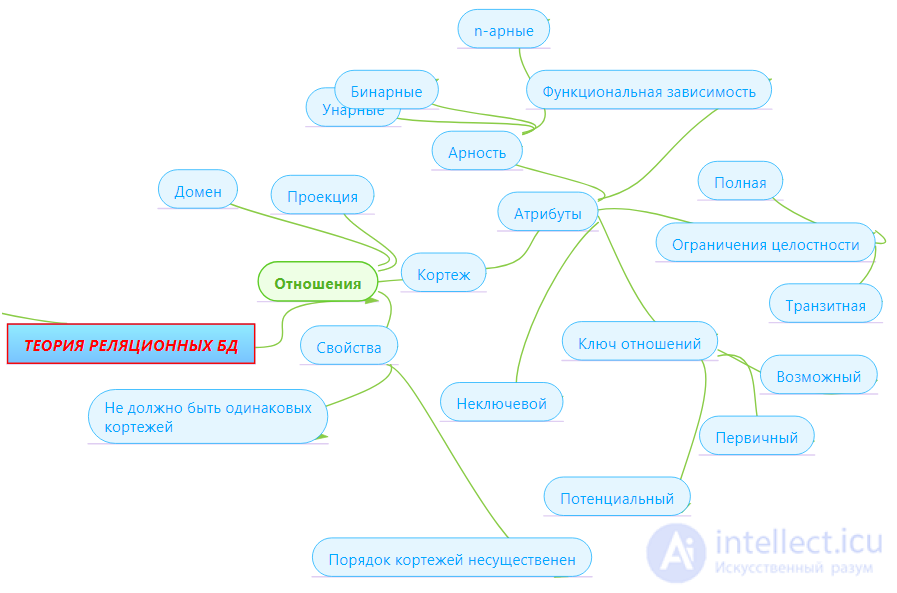
The concept of the first normal form has already been discussed in Chapter 2. The first normal form ( 1NF ) is a common relationship. According to our definition of relationships, any relationship is automatically already in 1NF. Let us briefly recall the properties of relations (these will be the properties of 1NF):
In the course of logical modeling, in the first step, it was proposed to store data in one respect, having the following attributes:
СОТРУДНИКИ_ОТДЕЛЫ_ПРОЕКТЫ ( Н_СОТР , ФАМ , Н_ОТД , ТЕЛ , Н_ПРО , ПРОЕКТ , Н_ЗАДАН )
Where
Н_СОТР - табельный номер сотрудника
ФАМ - фамилия сотрудника
Н_ОТД - номер отдела, в котором числится сотрудник
ТЕЛ - телефон сотрудника
Н_ПРО - номер проекта, над которым работает сотрудник
ПРОЕКТ - наименование проекта, над которым работает сотрудник
Н_ЗАДАН - номер задания, над которым работает сотрудник
Because каждый сотрудник в каждом проекте выполняет ровно одно задание, то в качестве потенциального ключа отношения необходимо взять пару атрибутов { Н_СОТР , Н_ПРО }.
В текущий момент состояние предметной области отражается следующими фактами:
Это состояние отражается в таблице (курсивом выделены ключевые атрибуты):
| Н_СОТР | ФАМ | Н_ОТД | ТЕЛ | Н_ПРО | PROJECT | Н_ЗАДАН |
|---|---|---|---|---|---|---|
| one | Ivanov | one | 11-22-33 | one | Space | one |
| one | Ivanov | one | 11-22-33 | 2 | Climate | one |
| 2 | Петров | one | 11-22-33 | one | Space | 2 |
| 3 | Сидоров | 2 | 33-22-11 | one | Space | 3 |
| 3 | Сидоров | 2 | 33-22-11 | 2 | Climate | 2 |
Таблица 1 Отношение СОТРУДНИКИ_ОТДЕЛЫ_ПРОЕКТЫ
Аномалии обновления
Даже одного взгляда на таблицу отношения СОТРУДНИКИ_ОТДЕЛЫ_ПРОЕКТЫ достаточно, чтобы увидеть, что данные хранятся в ней с большой избыточностью . Во многих строках повторяются фамилии сотрудников, номера телефонов, наименования проектов. Кроме того, в данном отношении хранятся вместе независимые друг от друга данные - и данные о сотрудниках, и об отделах, и о проектах, и о работах по проектам. Пока никаких действий с отношением не производится, это не страшно. Но как только состояние предметной области изменяется, то, при попытках соответствующим образом изменить состояние базы данных, возникает большое количество проблем.
Исторически эти проблемы получили название аномалии обновления . Попытки дать строгое понятие аномалии в базе данных не являются вполне удовлетворительными [51, 7]. В данных работах аномалии определены как противоречие между моделью предметной области и физической моделью данных, поддерживаемых средствами конкретной СУБД. "Аномалии возникают в том случае, когда наши знания о предметной области оказываются, по каким-то причинам, невыразимыми в схеме БД или входящими в противоречие с ней" [7]. Мы придерживаемся другой точки зрения, заключающейся в том, что аномалий в смысле определений упомянутых авторов нет, а есть либо неадекватность модели данных предметной области, либо некоторые дополнительные трудности в реализации ограничений предметной области средствами СУБД. Более глубокое обсуждение проблемы строгого определения понятия аномалий выходит за пределы данной работы.
Таким образом, мы будем придерживаться интуитивного понятия аномалии как неадекватности модели данных предметной области, (что говорит на самом деле о том, что логическая модель данных попросту неверна!) или как необходимости дополнительных усилий для реализации всех ограничений определенных в предметной области (дополнительный программный код в виде триггеров или хранимых процедур).
Because аномалии проявляют себя при выполнении операций, изменяющих состояние базы данных, то различают следующие виды аномалий:
В отношении СОТРУДНИКИ_ОТДЕЛЫ_ПРОЕКТЫ можно привести примеры следующих аномалий:
Аномалии вставки (INSERT)
В отношение СОТРУДНИКИ_ОТДЕЛЫ_ПРОЕКТЫ нельзя вставить данные о сотруднике, который пока не участвует ни в одном проекте. Действительно, если, например, во втором отделе появляется новый сотрудник, скажем, Пушников, и он пока не участвует ни в одном проекте, то мы должны вставить в отношение кортеж (4, Пушников, 2, 33-22-11, null, null, null). Это сделать невозможно, т.к. атрибут Н_ПРО (номер проекта) входит в состав потенциального ключа, и, следовательно, не может содержать null-значений.
Точно также нельзя вставить данные о проекте, над которым пока не работает ни один сотрудник.
Причина аномалии - хранение в одном отношении разнородной информации (и о сотрудниках, и о проектах, и о работах по проекту).
The conclusion is that the logical data model is inadequate to the domain model. A database based on this model will not work correctly.
Update Anomaly (UPDATE)
Фамилии сотрудников, наименования проектов, номера телефонов повторяются во многих кортежах отношения. Поэтому если сотрудник меняет фамилию, или проект меняет наименование, или меняется номер телефона, то такие изменения необходимо одновременно выполнить во всех местах, где эта фамилия, наименование или номер телефона встречаются, иначе отношение станет некорректным (например, один и тот же проект в разных кортежах будет называться по-разному). Таким образом, обновление базы данных одним действием реализовать невозможно. Для поддержания отношения в целостном состоянии необходимо написать триггер, который при обновлении одной записи корректно исправлял бы данные и в других местах.
Причина аномалии - избыточность данных, также порожденная тем, что в одном отношении хранится разнородная информация.
Conclusion - increases the complexity of database development. A database based on such a model will work correctly only if there is additional program code in the form of triggers.
Deletion Anomalies (DELETE)
When deleting some data, other information may be lost. For example, if you close the project "Cosmos" and delete all the lines in which it is found, then all data about the employee Petrov will be lost. If you remove the employee Sidorov, you will lose information that in the department number 2 is the telephone 33-22-11. If the project is temporarily suspended, then deleting the data on the work on this project will also delete the data on the project itself (project name). Moreover, if there was an employee who worked only on this project, then the data about that employee would be lost.
Причина аномалии - хранение в одном отношении разнородной информации (и о сотрудниках, и о проектах, и о работах по проекту).
Вывод - логическая модель данных неадекватна модели предметной области. База данных, основанная на такой модели, будет работать неправильно.
Функциональные зависимости
Отношение СОТРУДНИКИ_ОТДЕЛЫ_ПРОЕКТЫ находится в 1НФ, при этом, как было показано выше, логическая модель данных не адекватна модели предметной области. Таким образом, первой нормальной формы недостаточно для правильного моделирования данных.
Определение функциональной зависимости
Для устранения указанных аномалий (а на самом деле для правильного проектирования модели данных !) применяется метод нормализации отношений. Нормализация основана на понятии функциональной зависимости атрибутов отношения.
Определение 1 . Let be  - отношение. Множество атрибутов
  функционально зависимо от множества атрибутов
  ( функционально определяет ) тогда и только тогда, когда для любого состояния отношения для любых кортежей
  из того, что
  следует что
  (т.е. во всех кортежах, имеющих одинаковые значения атрибутов , значения атрибутов также совпадают в любом состоянии отношения ). Символически функциональная зависимость записывается
 .
.
The set of attributes is called the determinant of functional dependency , and the set of attributes is called the dependent part .
Comment.If attributes constitute a potential relationship key , then any relationship attribute is functionally dependent on .
Example 1 . In relation to the EMPLOYEES_DESIGNS_Projects , the following examples of functional dependencies can be given:
Attribute dependence on relationship key:
{ N_SOPR , N_PRO }  FAM
FAM
{ N_SOTR , N_PRO } N_OTD
{ H_SOTR , N_PRO } TEL
{ Н_СОТР , Н_ПРО } ПРОЕКТ
{ Н_СОТР , Н_ПРО } Н_ЗАДАН
Зависимость атрибутов, характеризующих сотрудника от табельного номера сотрудника:
Н_СОТР ФАМ
Н_СОТР Н_ОТД
Н_СОТР ТЕЛ
Зависимость наименования проекта от номера проекта:
Н_ПРО ПРОЕКТ
Зависимость номера телефона от номера отдела:
Н_ОТД ТЕЛ
Comment. Приведенные функциональные зависимости не выведены из внешнего вида отношения, приведенного в таблице 1. Эти зависимости отражают взаимосвязи, обнаруженные между объектами предметной области и являются дополнительными ограничениями, определяемыми предметной областью. Таким образом, функциональная зависимость - семантическое понятие . Она возникает, когда по значениям одних данных в предметной области можно определить значения других данных. Например, зная табельный номер сотрудника, можно определить его фамилию, по номеру отдела можно определить телефона. Функциональная зависимость задает дополнительные ограничения на данные, которые могут храниться в отношениях. Для корректности базы данных (адекватности предметной области) необходимо при выполнении операций модификации базы данных проверять все ограничения, определенные функциональными зависимостями.
Функциональные зависимости отношений и математическое понятие функциональной зависимости
Функциональная зависимость атрибутов отношения напоминает понятие функциональной зависимости в математике. Но это не одно и то же . Для сравнения напомним математическое понятие функциональной зависимости:
Определение 2 . Функциональная зависимость ( функция ) - это тройка объектов  where
where
 - множество ( область определения ),
 - множество ( множество значений ),
 - правило, согласно которому каждому элементу
  ставится в соответствие один и только один элемент
  ( правило функциональной зависимости ).
Функциональная зависимость обычно обозначается как  or
or  .
.
Comment. Rule может быть задано любым способом - в виде формулы (чаще всего), при помощи таблицы значений, при помощи графика, текстовым описанием и т.д.
Функциональная зависимость атрибутов отношения тоже напоминает это определение. Действительно:
(или декартово произведение доменов, если является множеством атрибутов) (или декартово произведение доменов) реализуется следующим алгоритмом - 1) по данному значению атрибута найти любой кортеж отношения, содержащий это значение, 2) значение атрибута в этом кортеже и будет значением функциональной зависимости, соответствующим данному . Определение функциональной зависимости в отношении гарантирует, что найденное значение не зависит от выбора кортежа , поэтому правило определено корректно.
Отличие от математического понятия отношения состоит в том, что, если рассматривать математическое понятие функции, то для фиксированного значения соответствующее значение функции всегда одно и то же . Например, если задана функция  , то для значения
  соответствующее значение
  всегда будет равно 4. В противоположность этому в отношениях значение зависимого атрибута может принимать различные значения в различных состояниях базы данных. Например, атрибут ФАМ функционально зависит от атрибута Н_СОТР . Предположим, что сейчас сотрудник с табельным номером 1 имеет фамилию Иванов, т.е. при значении детерминанта равного 1, значение зависимого аргумента равно "Иванов". Но сотрудник может сменить фамилию, например на "Сидоров". Теперь при том же значении детерминанта, равного 1, значение зависимого аргумента равно "Сидоров".
Таким образом, понятие функциональной зависимости атрибутов нельзя считать полностью эквивалентным математическому понятию функциональной зависимости, т.к. значение этой зависимости различны при разных состояниях отношения, и, самое главное, эти значения могут меняться непредсказуемо .
Функциональная зависимость атрибутов утверждает лишь то, что для каждого конкретного состояния базы данных по значению одного атрибута (детерминанта) можно однозначно определить значение другого атрибута (зависимой части). Но конкретные значение зависимой части могут быть различны в различных состояниях базы данных.
2НФ (Вторая Нормальная Форма)
Определение 3 . Отношение находится во второй нормальной форме ( 2НФ ) тогда и только тогда, когда отношение находится в 1НФ и нет неключевых атрибутов, зависящих от части сложного ключа . ( Неключевой атрибут - это атрибут, не входящий в состав никакого потенциального ключа).
Comment. Если потенциальный ключ отношения является простым, то отношение автоматически находится в 2НФ.
Отношение СОТРУДНИКИ_ОТДЕЛЫ_ПРОЕКТЫ не находится в 2НФ, т.к. есть атрибуты, зависящие от части сложного ключа:
Зависимость атрибутов, характеризующих сотрудника от табельного номера сотрудника является зависимостью от части сложного ключа:
Н_СОТР ФАМ
Н_СОТР Н_ОТД
Н_СОТР ТЕЛ
Зависимость наименования проекта от номера проекта является зависимостью от части сложного ключа:
Н_ПРО ПРОЕКТ
Для того, чтобы устранить зависимость атрибутов от части сложного ключа, нужно произвести декомпозицию отношения на несколько отношений. При этом те атрибуты, которые зависят от части сложного ключа, выносятся в отдельное отношение.
Отношение СОТРУДНИКИ_ОТДЕЛЫ_ПРОЕКТЫ декомпозируем на три отношения - СОТРУДНИКИ_ОТДЕЛЫ , ПРОЕКТЫ , ЗАДАНИЯ .
Отношение СОТРУДНИКИ_ОТДЕЛЫ ( Н_СОТР , ФАМ , Н_ОТД , ТЕЛ ):
Functional dependencies:
Зависимость атрибутов, характеризующих сотрудника от табельного номера сотрудника:
Н_СОТР ФАМ
Н_СОТР Н_ОТД
Н_СОТР ТЕЛ
Зависимость номера телефона от номера отдела:
Н_ОТД ТЕЛ
| H_SOTR | FAM | N_OTD | TEL |
|---|---|---|---|
| one | Ivanov | one | 11-22-33 |
| 2 | Petrov | one | 11-22-33 |
| 3 | Sidorov | 2 | 33-22-11 |
Table 2 Relationship EMPLOYEES_DEPARTMENTS
Attitude PROJECTS ( N_PRO , PROJECT ):
Functional dependencies:
N_PRO PROJECT
| N_PRO | PROJECT |
|---|---|
| one | Space |
| 2 | Climate |
Table 3 Attitudes PROJECTS
RELATIONSHIP TASKS ( N_SOPR , N_PRO , N_ZADAN ):
Functional dependencies:
{ Н_СОТР , Н_ПРО } N_ZADAN
| H_SOTR | N_PRO | N_ZADAN |
|---|---|---|
| one | one | one |
| one | 2 | one |
| 2 | one | 2 |
| 3 | one | 3 |
| 3 | 2 | 2 |
Table 4 Relationships TASKS
Analysis of decomposed relationships
Relations obtained as a result of decomposition are in 2NF. Indeed, the EMPLOYEES and PROJECTS relationships have simple keys, therefore they are automatically located in 2NF, the JOBS relation has a complex key, but the only non-key attribute N_ZADAN functionally depends on the entire key { Н_СОТР , Н_ПРО } .
Part of update anomalies resolved. So, data on employees and projects are now stored in different relationships, therefore, when employees who are not participating in any project appear, tuples are added to the EMPLOYEES_DEPARTMENTS relationship. Similarly, when a project appears that no employee is working on, a tuple is simply inserted into the PROJECTS relationship.
The names of employees and project names are now stored without redundancy. If the employee changes the name or the project changes the name, the update will be made in one place.
If the project is temporarily terminated, but the project itself is required to be preserved, then for this project the corresponding tuples are deleted for the TASK , and the data on the project itself and the data on the employees who participated in the project remain in the relationship PROJECTS and EMPLOYEES .
However, part of the anomalies could not be resolved.
The remaining insertion anomalies (INSERT)
In relation to EMPLOYEES_DEPARTMENTS, you cannot insert a tuple (4, Pushnikov, 1, 33-22-11), because at the same time, it turns out that two employees from the 1st Division (Ivanov and Pushnikov) have different telephone numbers, and this contradicts the domain model. In this situation, two solutions can be proposed, depending on what really happened in the subject area. Another phone number can be entered for two reasons - by mistake of the person entering the data about the new employee, or because the number in the department has really changed. Then you can write a trigger that, when inserting an employee record, checks whether the phone matches the already existing phone from another employee of the same department. If the numbers are different, the system should ask the question whether to leave the old number in the department or replace it with a new one. If you need to leave the old number (the new number is entered incorrectly), then the tuple with the data about the new employee will be inserted, but the phone number will be the one that already exists in the department (in this case, 11-22-33). If the number in the department has really changed, then the tuple will be inserted with the new number, and at the same time the phone numbers of all employees of the same department will be changed. And in that and in other case not to do without development of the bulky trigger.
The reason for the anomaly is data redundancy, due to the fact that in one respect heterogeneous information is stored (about employees and about departments).
Conclusion - increases the complexity of database development. A database based on such a model will work correctly only if there is additional program code in the form of triggers.
UPDATE Remaining Anomalies
The same phone numbers are repeated in many tuples of a relationship. Therefore, if a telephone number changes in a department, then such changes must be made simultaneously in all places where this telephone number is found, otherwise the attitude will become incorrect. Thus, updating the database with one action is impossible to implement. You need to write a trigger that, when updating one entry, correctly corrects phone numbers in other places.
The reason for the anomaly is data redundancy, also generated by the fact that heterogeneous information is stored in one respect.
Conclusion - increases the complexity of database development. A database based on such a model will work correctly only if there is additional program code in the form of triggers.
The remaining deletion anomalies (DELETE)
When deleting some data, other information may still be lost. For example, if you delete the employee Sidorov, you will lose the information that in the section number 2 is the telephone 33-22-11.
The reason for the anomaly is storing in one respect heterogeneous information (both about employees and about departments).
The conclusion is that the logical data model is inadequate to the domain model. A database based on this model will not work correctly.
Note that in the transition to the second normal form of the relationship became almost adequate subject area. There are also difficulties in developing a database associated with the need to write triggers that maintain the integrity of the database. These difficulties are now associated with only one relationship EMPLOYEES_DEPARTMENTS .
3NF (Third Normal Form)
Definition 4 . Attributes are called mutually independent if neither of them is functionally dependent on the other.
Definition 5 . Attitude is in the third normal form ( 3NF ) if and only if the relation is in 2NF and all non-key attributes are mutually independent .
The ratio EMPLOYEES_DESIGNS is not in 3NF, because there is a functional dependence of non-key attributes (the dependence of a telephone number on a department number):
N_OTD TEL
In order to eliminate the dependence of non-key attributes, it is necessary to decompose the relationship into several relations. In this case, those non-key attributes that are dependent, are taken out in a separate relationship.
Attitudes EMPLOYEES_DESETS we decompose into two relations - EMPLOYEES , DEPARTMENTS .
Attitude EMPLOYEES ( H_COTR , FAM , H_OTD ):
Functional dependencies:
The dependence of the attributes characterizing the employee from the employee's employee number:
H_SOTR FAM
H_SOTR N_OTD
H_SOTR TEL
| H_SOTR | FAM | N_OTD |
|---|---|---|
| one | Ivanov | one |
| 2 | Petrov | one |
| 3 | Sidorov | 2 |
Table 5 Attitude EMPLOYEES
Attitude DEPARTMENTS ( N_OTD , TEL ):
Functional dependencies:
Dependence of the telephone number on the department number:
N_OTD TEL
| N_OTD | TEL |
|---|---|
| one | 11-22-33 |
| 2 | 33-22-11 |
Table 6 Attitudes DEPARTMENTS
Note that the N_OTD attribute, which was not the key for EMPLOYEES , has become a potential key for the DEPARTMENT . This is due to this eliminated redundancy associated with multiple storage of the same phone numbers.
Conclusion. Thus, all detected update anomalies are eliminated. The relational model consisting of four relations EMPLOYEES , DEPARTMENTS , PROJECTS , TASKS , which are in the third normal form, is adequate to the described domain model, and requires only those triggers that maintain referential integrity. Such triggers are standard and do not require much effort in development.
Algorithm of normalization (reduction to 3NF)
So, the normalization algorithm (i.e., the algorithm for reducing relations to 3NF) is described as follows.
Step 1 (Reduction to 1NF) . In the first step, one or more relations are defined that reflect the concepts of the domain. According to the domain model (not in appearance of the obtained relationships!), The detected functional dependencies are written out. All relationships are automatically in 1NF.
Step 2 (Reduction to 2NF) . If in some respects the dependence of attributes on the part of a complex key is found, then we decompose these relations into several relations as follows: those attributes that depend on the part of the complex key are put into a separate relationship with this part of the key. In the original relationship, all key attributes remain:
Initial relationship: 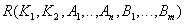 .
.
Key:  - complicated.
Functional dependencies:
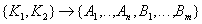 - dependence of all attributes on the relation key.
 - dependence of some attributes on a part of a complex key.
Decomposed relationships:
 - the remainder of the original relationship. Key .
 - attributes removed from the original relationship along with a part of a complex key. Key
  .
.
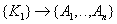
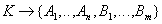
Step 3 (Reduction to 3NF) . If in some respects the dependence of some non-key attributes of other non-key attributes is detected, then we decompose these relations as follows: those non-key attributes that depend on other non-key attributes are taken to a separate relation. In the new relation, the determinant of functional dependence becomes the key:
Initial relationship: 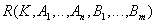 .
.
Key:  .
.
Functional dependencies:
 - dependence of all attributes on the relation key.
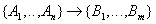 - dependence of some non-key attributes of other non-key attributes.
Decomposed relationships:
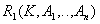 - the remainder of the original relationship. Key .
 - attributes removed from the original relationship along with the determinant of functional dependency. Key
  .
.
Comment. In practice, when creating a logical data model, as a rule, they do not directly follow the normalization algorithm. Experienced developers usually build relationships in 3NF right away. In addition, the main means of developing logical data models are various variants of ER-diagrams. The peculiarity of these diagrams is that they immediately allow you to create relationships in 3NF. However, the above algorithm is important for two reasons. First , this algorithm shows what problems arise when developing weakly normalized relations. Secondly , as a rule, the domain model is never properly developed from the first step. The domain experts may forget about something, the developer may misunderstand the expert, the rules adopted in the domain may change during the development, etc. All this may lead to the emergence of new dependencies that were absent in the original domain model. Here it is just necessary to use the normalization algorithm at least in order to make sure that the relations remain in 3NF and the logical model has not deteriorated.
Criteria Analysis for Normalized and Unnormalized Data Models
Comparison of normalized and non-normalized models
Let us put together the results of the analysis of the criteria by which we wanted to evaluate the impact of logical data modeling on the quality of physical data models and database performance:
| Criterion | Relationships are poorly normalized. (1NF, 2NF) |
Relationships are strongly normalized. (3NF) |
|---|---|---|
| Adequacy of the domain database | WORSE (-) | BETTER (+) |
| Ease of database development and maintenance | MORE DIFFICULT (-) | EASIER (+) |
| The speed of the insert, update, delete | SLOWER (-) | FASTER (+) |
| The speed of data sampling | FASTER (+) | SLOWER (-) |
As can be seen from the table, the more strongly normalized relations turn out to be better designed (three pluses, one minus). They are more relevant to the subject area, easier to develop, for them faster database modification operations are performed. True, this is achieved at the cost of some deceleration of data sampling operations.
For weakly normalized relations, the only advantage is that if the database is addressed only with requests for data sampling, then for weakly normalized relations such requests are executed faster. This is due to the fact that in such a relationship the connection of the relations has already been made, and time is not wasted on sampling the data.
Thus, the choice of the degree of normalization of relations depends on the nature of the requests that are most often addressed to the database.
OLTP and OLAP systems
There are some classes of systems for which strongly or weakly normalized data models are more suitable.
Strongly normalized data models are well suited for so-called OLTP applications ( On-Line Transaction Processing ( OLTP ) - online transaction processing ). Typical examples of OLTP applications are warehouse accounting systems, ticket booking systems, banking systems that perform money transfer operations, etc. The main function of such systems is to perform a large number of short transactions. The transactions themselves look relatively simple, for example, "withdraw the amount of money from account A, add this amount to account B". The problem is that, firstly, there are a lot of transactions, secondly, they are executed simultaneously (several thousand concurrent users can be connected to the system), thirdly, if an error occurs, the transaction must completely roll back and return the system to the state that was before the start of the transaction (there should not be a situation when money is withdrawn from account A, but not credited to account B). Almost all database queries in OLTP applications consist of insert, update, delete commands. Sampling requests are primarily intended to allow users to select from various directories. Most requests are thus known in advance at the stage of system design. Thus, the speed and reliability of short data update operations is critical for OLTP applications. The higher the level of data normalization in an OLTP application, so it is usually faster and more reliable. Deviations from this rule can occur when, even at the development stage, some frequently occurring queries are known that require connection of relations and the performance of which depends greatly on the performance of applications. In this case, you can sacrifice normalization to speed up the execution of such requests.
Another type of application is the so-called OLAP-applications ( On-Line Analitical Processing ( OLAP ) - operational analytical data processing ). This is a generic term describing the principles of building decision support systems ( DSS ), data warehouses, data mining systems . Such systems are designed to find the dependencies between the data (for example, you can try to determine how the sales of goods are related to the characteristics of potential buyers), to conduct a what-if analysis. OLAP applications operate on large amounts of data already accumulated in OLTP applications, taken from spreadsheets or from other data sources. Such systems are characterized by the following features:
The data of OLAP applications are usually represented as one or several hypercubes, the measurements of which are reference data, and the data itself is stored in the cells of the hypercube itself. For example, you can build a hypercube, the dimensions of which are: time (in quarters, years), the type of product and the separation of the company, and sales volumes are stored in cells. Such a hypercube will contain data on sales of various types of goods by quarters and divisions. Based on this data, you can answer questions like "which division has the best sales volumes in the current year?", Or "what are the sales trends of the South-West regions in the current year compared to the previous year?"
Physically, a hypercube can be built on the basis of a special multidimensional data model ( MOLAP - Multidimensional OLAP ) or built by means of a relational data model ( ROLAP - Relational OLAP ).
Возвращаясь к проблеме нормализации данных, можно сказать, что в системах OLAP, использующих реляционную модель данных (ROLAP), данные целесообразно хранить в виде слабо нормализованных отношений, содержащих заранее вычисленные основные итоговые данные. Большая избыточность и связанные с ней проблемы тут не страшны, т.к. обновление происходит только в момент загрузки новой порции данных. При этом происходит как добавление новых данных, так и пересчет итогов.
Корректность процедуры нормализации - декомпозиция без потерь. Теорема Хеза
Как было показано выше, алгоритм нормализации состоит в выявлении функциональных зависимостей предметной области и соответствующей декомпозиции отношений. Предположим, что мы уже имеем работающую систему, в которой накоплены данные. Пусть данных корректны в текущий момент, т.е. факты предметной области правильно отражаются текущим состоянием базы данных. Если в предметной области обнаружена новая функциональная зависимость (либо она была пропущена на этапе моделирования предметной области, либо просто изменилась предметная область), то возникает необходимость заново нормализовать данные. При этом некоторые отношения придется декомпозировать в соответствии с алгоритмом нормализации. Возникают естественные вопросы - что произойдет с уже накопленными данными? Не будут ли данные потеряны в ходе декомпозиции? Можно ли вернуться обратно к исходным отношениям, если будет принято решение отказаться от декомпозиции, восстановятся ли при этом данные?
Для ответов на эти вопросы нужно ответить на вопрос - что же представляет собой декомпозиция отношений с точки зрения операций реляционной алгебры? При декомпозиции мы из одного отношения получаем два или более отношений, каждое из которых содержит часть атрибутов исходного отношения. В полученных новых отношениях необходимо удалить дубликаты строк, если таковые возникли. Это в точности означает, что декомпозиция отношения есть не что иное, как взятие одной или нескольких проекций исходного отношения так, чтобы эти проекции в совокупности содержали (возможно, с повторениями) все атрибуты исходного отношения. Т.е., при декомпозиции не должны теряться атрибуты отношений. Но при декомпозиции также не должны потеряться и сами данные. Данные можно считать не потерянными в том случае, если возможна обратная операция - по декомпозированным отношениям можно восстановить исходное отношение в точности в прежнем виде . Операцией, обратной операции проекции, является операция соединения отношений. Имеется большое количество видов операции соединения (см. гл. 4). Because при восстановлении исходного отношения путем соединения проекций не должны появиться новые атрибуты, то необходимо использовать естественное соединение .
Определение 6 . Projection  relations на множество атрибутов называется собственной , если множество атрибутов является собственным подмножеством множества атрибутов отношения (т.е. множество атрибутов не совпадает с множеством всех атрибутов отношения ).
Определение 7 . Собственные проекции  and
and  relations называются декомпозицией без потерь , если отношение точно восстанавливается из них при помощи естественного соединения для любого состояния отношения :
 .
.
Рассмотрим пример, показывающий, что декомпозиция без потерь происходит не всегда.
Пример 2 . Пусть дано отношение :
| НОМЕР | ФАМИЛИЯ | ЗАРПЛАТА |
|---|---|---|
| one | Ivanov | 1000 |
| 2 | Петров | 1000 |
Таблица 7 Отношение
Рассмотрим первый вариант декомпозиции отношения на два отношения:
| НОМЕР | ЗАРПЛАТА |
|---|---|
| one | 1000 |
| 2 | 1000 |
Таблица 8 Отношение
| ФАМИЛИЯ | ЗАРПЛАТА |
|---|---|
| Ivanov | 1000 |
| Петров | 1000 |
Таблица 9 Отношение
Естественное соединение этих проекций, имеющих общий атрибут "ЗАРПЛАТА", очевидно, будет следующим (каждая строка одной проекции соединится с каждой строкой другой проекции):
| НОМЕР | ФАМИЛИЯ | ЗАРПЛАТА |
|---|---|---|
| one | Ivanov | 1000 |
| one | Петров | 1000 |
| 2 | Ivanov | 1000 |
| 2 | Петров | 1000 |
Таблица 10 Отношение 
Итак, данная декомпозиция не является декомпозицией без потерь, т.к. исходное отношение не восстанавливается в точном виде по проекциям (серым цветом выделены лишние кортежи).
Рассмотрим другой вариант декомпозиции:
| НОМЕР | ФАМИЛИЯ |
|---|---|
| one | Ivanov |
| 2 | Петров |
Таблица 11 Отношение
| НОМЕР | ЗАРПЛАТА |
|---|---|
| one | 1000 |
| 2 | 1000 |
Таблица 12 Отношение
По данным проекциям, имеющие общий атрибут "НОМЕР", исходное отношение восстанавливается в точном виде. Тем не менее, нельзя сказать, что данная декомпозиция является декомпозицией без потерь, т.к. мы рассмотрели только одно конкретное состояние отношения , и не можем сказать, будет ли и в других состояниях отношение восстанавливаться точно. Например, предположим, что отношение перешло в состояние:
| НОМЕР | ФАМИЛИЯ | ЗАРПЛАТА |
|---|---|---|
| one | Ivanov | 1000 |
| 2 | Петров | 1000 |
| 2 | Сидоров | 2000 |
Таблица 13 Отношение
Кажется, что этого не может быть, т.к. значения в атрибуте "НОМЕР" повторяются. Но мы же ничего не говорили о ключе этого отношения! Сейчас проекции будут иметь вид:
| НОМЕР | ФАМИЛИЯ |
|---|---|
| one | Ivanov |
| 2 | Петров |
| 2 | Сидоров |
Таблица 14 Отношение
| НОМЕР | ЗАРПЛАТА |
|---|---|
| one | 1000 |
| 2 | 1000 |
| 2 | 2000 |
Таблица 15 Отношение
Естественное соединение этих проекций будет содержать лишние кортежи:
| НОМЕР | ФАМИЛИЯ | ЗАРПЛАТА |
|---|---|---|
| one | Ivanov | 1000 |
| 2 | Петров | 1000 |
| 2 | Петров | 2000 |
| 2 | Сидоров | 1000 |
| 2 | Сидоров | 2000 |
Таблица 16 Отношение
Conclusion. Таким образом, без дополнительных ограничений на отношение нельзя говорить о декомпозиции без потерь.
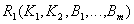
Такими дополнительными ограничениями и являются функциональные зависимости. Имеет место следующая теорема Хеза [54]:
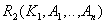
Теорема (Хеза) . Let be  является отношением, и
  - атрибуты или множества атрибутов этого отношения. Если имеется функциональная зависимость
  , то проекции
  and
and  образуют декомпозицию без потерь.
Proof . Необходимо доказать, что для любого состояния отношения . В левой и правой части равенства стоят множества кортежей, поэтому для доказательства достаточно доказать два включения для двух множеств кортежей:  and
and  .
.
Докажем первое включение . Возьмем произвольный кортеж  . Докажем, что он включается также и в
  . По определению проекции, кортежи
  and
and  . По определению естественного соединения кортежи
  and
and  , имеющие одинаковое значение
  общего атрибута
  , будут соединены в процессе естественного соединения в кортеж
  . Таким образом, включение доказано.
Докажем обратное включение . Возьмем произвольный кортеж  . Докажем, что он включается также и в
  . По определению естественного соединения получим, что в имеются кортежи and . Because , то существует некоторое значение
  , такое что кортеж
  . Аналогично, существует некоторое значение
  , такое что кортеж
  . Кортежи
  and
and  имеют одинаковое значение атрибута
  , равное
  . Из этого, в силу функциональной зависимости , следует, что
  . Таким образом, кортеж
  . Обратное включение доказано. Теорема доказана .
Comment. В доказательстве теоремы Хеза наличие функциональной зависимости не использовалось при доказательстве включения . Это означает, что при выполнении декомпозиции и последующем восстановлении отношения при помощи естественного соединения, кортежи исходного отношения не будут потеряны . Основной смысл теоремы Хеза заключается в доказательстве того, что при этом не появятся новые кортежи , отсутствовавшие в исходном отношении.
Because алгоритм нормализации (приведения отношений к 3НФ) основан на имеющихся в отношениях функциональных зависимостях, то теорема Хеза показывает, что алгоритм нормализации является корректным, т.е. в ходе нормализации не происходит потери информации .
findings
При разработке базы данных можно выделить несколько уровней моделирования:
Ключевые решения, определяющие качество будущей базы данных закладываются на этапе разработки логической модели данных. "Хорошие" модели данных должны удовлетворять определенным критериям:
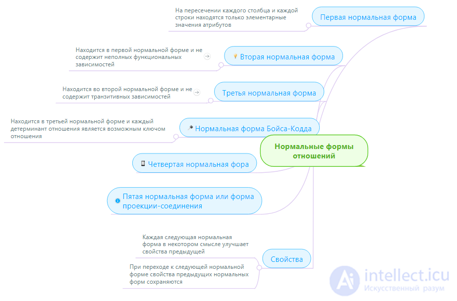
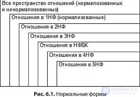
Первая нормальная форма ( 1НФ ) - это обычное отношение. Отношение в 1НФ обладает следующими свойствами:
Отношения, находящиеся в 1НФ являются "плохими" в том смысле, что они не удовлетворяют выбранным критериям - имеется большое количество аномалий обновления, для поддержания целостности базы данных требуется разработка сложных триггеров.
Отношение находится во второй нормальной форме ( 2НФ ) тогда и только тогда, когда отношение находится в 1НФ и нет неключевых атрибутов, зависящих от части сложного ключа.
Отношения в 2НФ "лучше", чем в 1НФ, но еще недостаточно "хороши" - остается часть аномалий обновления, по-прежнему требуются триггеры, поддерживающие целостность базы данных.
Отношение находится в третьей нормальной форме ( 3НФ ) тогда и только тогда, когда отношение находится в 2НФ и все неключевые атрибуты взаимно независимы.
Отношения в 3НФ являются самыми "хорошими" с точки зрения выбранных нами критериев - устранены аномалии обновления, требуются только стандартные триггеры для поддержания ссылочной целостности.
Переход от ненормализованных отношений к отношениям в 3НФ может быть выполнен при помощи алгоритма нормализации . Алгоритм нормализации заключается в последовательной декомпозиции отношений для устранения функциональных зависимостей атрибутов от части сложного ключа (приведение к 2НФ) и устранения функциональных зависимостей неключевых атрибутов друг от друга (приведение к 3НФ).
Корректность процедуры нормализации (декомпозиция без потери информации) доказывается теоремой Хеза .

Comments
To leave a comment
Databases, knowledge and data warehousing. Big data, DBMS and SQL and noSQL
Terms: Databases, knowledge and data warehousing. Big data, DBMS and SQL and noSQL