Lecture
Multidimensional models consider data either as facts with appropriate numerical parameters, or as textual measurements that characterize these facts. In retail, for example, a purchase is a fact, the purchase volume and cost are parameters, and the type of product purchased, the time and place of purchase are measurements. Requests aggregate parameter values over the entire measurement range, and as a result, values such as the total monthly sales of this product are obtained. Multidimensional data models have three important application areas related to data analysis issues.
Researchers proposed formal mathematical models of multidimensional databases, and then these proposals were refined in a specific software tool that implements these models [1, 2]. The box “The history of the development of multidimensional databases” describes the evolution of the multidimensional data model.
Spreadsheets, similar to those shown in Table 1, are a convenient tool for analyzing sales data: what products are sold, how many deals are made, and where. The main table (pivot table) is a two-dimensional spreadsheet with corresponding intermediate and final results, which is used to view more complex data by nesting several dimensions along the x and y axes and display data on several pages. The main tables usually support an iterative selection of data subsets and a change in the level of detail displayed.
Spreadsheets are not suitable for managing and storing multidimensional data because they too tightly link data to their appearance without separating structural information from the desired presentation of information. Say, adding a third dimension, such as time, or grouping data by generic product types requires a much more complex setup. The obvious solution is to use a separate spreadsheet for each dimension. But such a decision is justified only to a limited extent, since the analysis of such sets of tables quickly becomes too cumbersome.
Using databases that support SQL significantly increases the flexibility of handling structured data. However, to formulate many calculations, such as aggregates (sales for the year to the current moment), a combination of final and intermediate results, ranking, for example, determining the ten best-selling products, using the standard SQL variant is very difficult, if possible. When rearranging rows and columns, you must manually specify and combine different views. SQL extensions, such as the data cube operator [3] and query windows [4], partially solve these problems; in general, the pure relational model does not allow working with hierarchical dimensions at an acceptable level.
Spreadsheets and relational databases adequately handle datasets that have a small number of dimensions, but they do not fully meet the requirements of in-depth data analysis. The solution is to use technology that supports the full range of multi-dimensional data modeling tools.
Multidimensional databases treat data as cubes, which are the generalization of spreadsheets to any number of dimensions. In addition, cubes maintain a hierarchy of dimensions and formulas without duplicating their definitions. A set of corresponding cubes constitutes a multidimensional database (or data store).
Cubes are easy to manage by adding new measurement values. In common usage, this term denotes a figure with three dimensions, but theoretically a cube can have any number of dimensions. In practice, most often data cubes have from 4 to 12 dimensions [5, 6]. Modern tools often face a lack of performance when the so-called hypercube has over 10-15 measurements.
Combinations of dimension values define cube cells. Depending on the specific application, cells in a cube can be arranged both separately and densely. Cubes, as a rule, become fragmented as the number of dimensions increases and the degree of detail of measurement values increases.
In fig. 1 shows a cube containing data on sales in two Danish cities listed in table 1 with an additional dimension - “Time”. The corresponding cells store sales data. In the example, you can find the "fact" - a non-empty cell containing the corresponding numerical parameters - for each combination time, product and city, where at least one sale was made. The cell contains the numerical values associated with the fact — in this case, this sales volume is the only parameter.
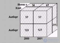 |
| Fig. 1. An example of a cube containing sales data. In this case, the cube summarizes the spreadsheet from Table 1, adding a third dimension to it - time |
In the general case, a cube allows you to present only two or three dimensions at a time, but you can also show more by investing one dimension in another. Thus, by projecting a cube onto a two- or three-dimensional space, you can reduce the dimension of the cube by aggregating some dimensions, which leads to working with more complex parameter values. For example, considering sales by city and time, we aggregate information for each combination city and time. So, on fig. 1, adding the fields 127 and 211, we get the total sales for Copenhagen in 2001.
Measurement is a key concept for multidimensional databases. Multivariate modeling involves the use of measurements to provide the maximum possible context for the facts [5]. Unlike relational databases, controlled redundancy in multidimensional databases is generally considered justified if it increases the information value. Since data in a multidimensional cube is often collected from other sources, for example, from a transactional system, the redundancy problems associated with updates can be solved much easier. As a rule, there is no redundancy in facts, it is only in dimensions.
Measurements are used to select and aggregate data at the required level of detail. Measurements are organized into a hierarchy consisting of several levels, each of which represents the level of detail required for the corresponding analysis.
Sometimes it is useful to define several hierarchies for a dimension. For example, a model can determine time in both fiscal and calendar years. Several hierarchies share one or more common, lowest levels, for example, day and month, and the model groups them into several higher levels — the fiscal quarter and the calendar quarter. To avoid duplicate definitions, multidimensional database metadata define a hierarchy of dimensions.
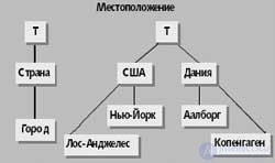 |
| Fig. 2. An example of a location measurement scheme. Each dimension value is part of the T value. |
In fig. 2 shows the “Location” scheme for sales data from Table 1. Of the three levels of location measurements, the lowest is the “City”. Values of the “City” level are grouped into values at the “Country” level, for example, Aalborg and Copenhagen are located in Denmark. Level T represents all measurements.
In some multidimensional models, a layer has several related properties that contain simple, non-hierarchical information. For example, “Package Size” may be a level property in the “Product” dimension. The packet size measurement can also receive this information. Using the property mechanism does not increase the number of dimensions in the cube.
Unlike the linear spaces that matrix algebra deals with, multidimensional models, as a rule, do not provide ordering functions or distances for measurement values. The only “ordering” is that the values of the higher level contain the values of the lower levels. However, for some dimensions, such as time, the ordering of dimension values can be used to calculate cumulative information, such as total sales for a certain period. Most models require the definition of a hierarchy of dimensions to form balanced trees — hierarchies must have the same height along all branches, and each value of the non-root level must have only one parent.
Facts represent a subject — some kind of pattern or event that needs to be analyzed. In most multidimensional data models, facts are uniquely determined by a combination of measurement values; a fact exists only when the cell for a particular combination of values is not empty. However, some models interpret the facts as “first class objects” with special properties. Most multidimensional models also require that each fact correspond to a single value at the lower level of each dimension, but in some models this is not a requirement [1].
Each fact has a certain granularity, a certain level from which a combination of measurement values is created. For example, the granularity of the fact in the cube presented in Fig. 1 is (Year x Product x City). (Year x Type x City) and (Day x Product x City) are respectively coarser and finer granularity.
Data warehouses, as a rule, contain the following three types of facts [5].
The data store often contains all three types of facts. The same basic data, for example, the movement of goods in a warehouse, can be contained in three different types of cubes: the flow of goods in the warehouse, the list of goods and the flow for the year to the current date.
Parameters consist of two components:
In a multidimensional database, the parameters, as a rule, represent the properties of the fact that the user wants to study. Parameters take on different values for different combinations of measurements. The property and formula are selected to represent a meaningful value for all combinations of aggregation levels. Since metadata defines a formula, data, unlike the case of spreadsheets, is not replicated.
In the calculations, the three different classes of parameters behave quite differently.
Additive and non-additive parameters can describe facts of any kind, while semi-additive parameters are usually used with snapshots or cumulative snapshots.
A multidimensional database is naturally designed for certain types of queries.
Multidimensional databases are implemented in two basic forms.
MOLAP systems, as a rule, allow to achieve more efficient use of disk space, as well as a shorter response time when processing requests.
The sidebar “Reducing response time when processing requests” describes some of the techniques used for this purpose. ROLAP systems tend to scale better with an increase in the number of facts they can store (although some MOLAP tools are now becoming more scalable), more flexible in terms of redefining cubes, and better support frequent updates. The merits of the two approaches are combined in a hybrid solution, in which MOLAP technology is used to store higher-level aggregated data, and detailed data are placed in ROLAP systems.
ROLAP, as a rule, uses star and snowflake schemes [5], in which data is stored in fact tables and measurement tables. The fact table contains one row for each fact in the cube. For each dimension, there is a separate column containing the parameter value for a particular fact, as well as a column for each dimension, which contains a foreign key that refers to the dimension table for a specific dimension.
The star and snowflake schemes differ in how they support measurements, and the choice between them mainly depends on what properties the developed system should have. As shown in fig. 3, in the “star” scheme, one table is assigned to each dimension. The dimension table contains a key column, one column for each dimension level with text descriptions of the values of this level, and one column for each level property in the dimension.
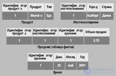 |
| Fig. 3. Star scheme for the sales cube. Information from all levels in the dimension is stored in one dimension table, for example, product names and product types are stored in the “Product” table |
Таблица фактов в схеме «звезда» в нашем примере содержит цены продаж для одной конкретной продажи и соответствующие значения измерений. Она включает столбец внешнего ключа для каждого из трех измерений: продукт, местоположение и время. Таблицы измерений имеют соответствующие ключевые столбцы и по одному столбцу для каждого уровня измерений, например, «Идентификатор местоположения», «Город» и «Страна». Для уровня T столбца не требуется, поскольку в нем всегда содержится одно и то же значение. Столбец ключа таблицы измерений, как правило, представляет собой искусственный целочисленный ключ без какой-либо семантики. Это позволяет избежать некорректной трактовки ключей, обеспечить более эффективное использование памяти и лучшую поддержку обновлений измерений, чем при работе с информативными ключами, получаемыми из систем-источников [5].
На более высоком уровне данных возникнет избыточность. Например, поскольку в мае 2001 года 31 день, значение 2001 будет повторено 31 раз. Поскольку измерения, как правило, занимают 1-5% всего пространства, требуемого для хранения куба, такая избыточность не вызывает нехватки памяти. Кроме того, централизованная поддержка обновления измерений гарантирует согласованность. Таким образом, использование денормализованных таблиц измерений, необходимых для поддержки упрощенного формулирования запросов, которые к тому же эффективно вычисляются, часто дает дополнительные преимущества.
Схема «снежинка» содержит по одной таблице для каждого уровня измерений, избегая избыточности, что может оказаться весьма полезным в некоторых ситуациях. Каждая из таблиц измерений содержит ключ, столбец с текстовыми описаниями значений уровней, возможно, столбцы для свойств уровней. Таблицы более низких уровней могут также содержать внешний ключ для доступа к более высокому уровню. Например, таблица дней на рис. 4 содержит целочисленный ключ, дату и внешний ключ для связи с таблицей месяцев.
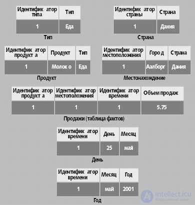 |
| Fig. 4. Схема «снежинка» для куба продаж. Информация из различных уровней в измерении хранится в различных таблицах. Например, названия продуктов и типы продуктов хранятся в таблицах «Продукт» и «Тип» соответственно |
Традиционные многомерные модели данных и методы их реализации предполагают, что:
Если эти предположения не выполняются, то стандартные модели и системы оказываются неадекватными. Особенно серьезные проблемы вызывают комплексные многомерные данные, поскольку они не являются суммируемыми (summarizable) — агрегированные результаты более высокого уровня нельзя получить из агрегированных результатов более низкого уровня. Запросы по результатам более низкого уровня будут приносить неверные данные, или предварительные вычисления, сохранение и последующее использование их результатов в данном случае невозможны. Вместо этого агрегированные результаты должны вычисляться непосредственно из базовых данных, что значительно увеличивает затраты на вычисления.
Суммирование требует применения распределенных агрегированных функций и значений иерархии измерений [1, 7]. Неформально иерархия измерений является «строгой», если ни одно из значений измерений не имеет более одного прямого родителя, «сюрьективной» (onto), если иерархия сбалансирована, и «покрывающей» (covering), если ни один локальный путь не «перескакивает» через уровень. Интуитивно это значит, что иерархии измерений должны быть сбалансированными деревьями. As shown in fig. 5, в случае нерегулярных иерархий измерений некоторые значения более низкого уровня при повторном использовании промежуточных результатов запросов будут либо посчитаны дважды, либо ни разу.
Нерегулярные иерархии возникают в разных приложениях, в том числе в иерархии административных структур [8], иерархии медицинских диагнозов [9] и иерархии концепций для Web-порталов, подобных Yahoo. Одно из решений — нормализовать нерегулярные иерархии, процесс, который предусматривает пополнение несюрьективных и непокрывающих иерархий фиктивными значениями измерений, и перестраивает наборы родителей, для того чтобы решить проблемы нестрогих иерархий. Это преобразование может выполняться прозрачным для пользователя образом [10].
За 30 лет с момента своего возникновения технология многомерных баз данных прошла серьезную эволюцию. С недавних пор она стала реализовываться в решениях, предназначенных для массового рынка, а ведущие производители теперь выпускают многомерные ядра вместе со своими реляционными базами данных, причем часто без дополнительной оплаты. Многомерная технология стала значительно более масштабируемой и зрелой.
Это порождает несколько важных тенденций. Данные, которые необходимо анализировать, становятся все более распределенными. К примеру, это часто необходимо для выполнения анализа, при котором используются данные в формате XML, получаемые с определенных Web-сайтов. Растущая распределенность данных, в свою очередь, требует применения методов, которые позволяют легко добавлять новые данные в многомерные базы данных, тем самым, упрощая задачу создания интегрированного хранилища данных. Среди примеров — автоматическая генерация измерений и кубов из новых источников данных и методы простой и динамической очистки данных.
Технология многомерных баз данных также применяется к новым типам данных, которые современные технологии зачастую не в состоянии адекватно анализировать. К примеру, классические методики, такие как предагрегирование не могут гарантировать небольшое время ответа на запросы, если данные постоянно меняются, как это происходит, например, когда информация поступает с датчиков или от движущихся объектов, таких как автомобили, оснащенные средствами глобального позиционирования.
Наконец, технология многомерных баз данных все больше будет применяться там, где результаты анализа напрямую передаются в другие системы, тем самым, исключая участие человека в этом процессе. Этот контекст в совокупности с необходимостью постоянного обновления предъявляет более жесткие требования к производительности, которым не удовлетворяет современная технология.
Торбен Бэч Педерсон (tbp@cs.auc.dk) — адъюнкт-профессор информатики университета Аалборга (Дания). К области его научных интересов относятся многомерные базы данных, OLAP, хранилища данных, федеративные базы данных и службы с учетом местоположения.
Кристиан Йенсен (csj@cs.auc.dk) — профессор информатики университета Аалборга. Он специализируется на проблематике многомерных баз данных, хранилищ данных, временных и пространственно-временных баз данных, а также службах с учетом местоположения.
Источником для многомерных баз данных послужили не современные технологии баз данных, а алгебра многомерных матриц, которая использовалась для ручного анализа данных с конца XIX столетия.
В конце 60-х годов компании IRI Software и Comshare независимо друг от друга начали разрабатывать то, что позднее стали называть системами управления многомерными базами данных. IRI Express, популярный в конце 70-х и начале 80-х годов инструментарий маркетингового анализа, стал лидером рынка средств оперативной аналитической обработки и был куплен корпорацией Oracle. На базе системы Comshare был создан инструментарий System W, в 80-х годах активно применявшийся для финансового планирования, анализа и формирования отчетов.
Образованная в 1991 году компания Arbor Software (теперь Hyperion Solutions) в качестве своей специализации выбрала создание многопользовательских серверов многомерных баз данных; результатом этих работ стала система Essbase. Позже Arbor лицензировала базовую версию Essbase корпорации IBM, которая интегрировала ее в DB2.
В 1993 году Э.Ф. Кодд ввел термин OLAP [1]. В начале 90-х сложилась еще одна важная концепция — крупные хранилища данных, которые, как правило, базируются на схемах «звезда» и «снежинка». При таком подходе для реализации многомерных баз удается использовать технологию реляционных баз данных.
В 1998 году корпорация Microsoft выпустила OLAP Server, первую многомерную систему, предназначенную для массового рынка, и теперь такие системы становятся распространенными продуктами и предлагаются без дополнительной оплаты вместе с популярными системами управления реляционными базами данных.
1. EF Codd, SB Codd, CT Salley, «Providing OLAP (On-Line Analytical Processing) to User-Analysts: An IT Mandate»,www.hyperion.com/solutions/whitepapers.cfm
backwards
Самые важные методы увеличения производительности в многомерных базах данных — это предвычисления (precomputation). Их специализированный аналог — предагрегирование (preaggregation), которое позволяет сократить время ответа на запросы, охватывающие потенциально огромные объемы данных, в степени, достаточной для проведения интерактивного анализа данных.
Вычисление и сохранение, или «материализация», сводных объемов продаж по странам и месяцам, — пример предагрегирования. Такой подход позволяет быстро получать ответы на запросы, касающиеся общего объема продаж, к примеру, в одном месяце, в одной стране или по кварталу и стране одновременно. Эти ответы можно получить из предварительно вычисленных данных и нет необходимости обращаться к информации, размещенной в хранилище данных.
Modern commercial relational databases, as well as specialized multidimensional systems, contain tools for optimizing queries based on pre-computed aggregates (aggregate) and automatic recomputation of stored aggregates when updating baseline data [1].
Full pre-aggregation — materialization of all combinations of aggregates — is impossible, since it requires too much disk space and time for preliminary calculations. Instead, modern OLAP systems follow a more practical approach to pre-aggregation, materializing only selected combinations of aggregates, and then using them to more efficiently calculate other aggregates [2]. Reuse of aggregates requires maintaining a valid multidimensional data structure.

Comments
To leave a comment
Databases, knowledge and data warehousing. Big data, DBMS and SQL and noSQL
Terms: Databases, knowledge and data warehousing. Big data, DBMS and SQL and noSQL