Analyzing queries to improve their execution speed - Tuning the

Это окончание невероятной информации про производительность запросов к хранилищу данных.

...

margin-right:0px">

If the histogram was built using a sample, the values RANGE_ROWS, EQ_ROWS, DISTINCT_RANGE_ROWS, and AVG_RANGE_ROWS will be estimates and therefore will not be whole numbers.

Density is information about the number of duplicates in the column or combination of columns being analyzed, and it is calculated as: 1 / (number of distinct values). When a column is used in an equality predicate, the number of qualifying rows is estimated using the density value obtained from the histogram. Histograms are also needed to estimate the selectivity of predicates in selections involving inequalities, joins, and other operators.

In addition to the timestamp (showing when the statistical data was collected), the number of rows in the table, the number of rows sampled for building the histogram, the density, the informational and average key length, and the histogram itself, the statistical information for a single column also includes an All density value, computed for each set of columns and defining the prefix of the column statistics set. This value can be seen in the second block of rows output by the DBCC SHOW_STATISTICS command. All density is an estimate of: 1 / (number of distinct values in the column prefix set). The meaning of this value is explained in the next paragraph.

Each multi-column statistics set (a histogram and two or more density values) is stored in a single statblob together with the timestamp of the last statistics update, the number of rows in the typical sample used for collecting statistics, the number of histogram steps, and the average key length. A string summary is created only for the first column, if it contains character data.

sp_helpindex and sp_helpstats show the lists of statistics available for the table being analyzed. sp_helpindex shows all indexes of the table, while sp_helpstats shows a list of all statistics on the table. Every index also has statistical information for its columns. Statistical information created using the CREATE STATISTICS command is equivalent to the statistics generated by the CREATE INDEX command, if the index is created on the same columns. The only difference is that CREATE STATISTICS will use the default sampling, while for CREATE INDEX statistics collection will be accompanied by a full table scan, since building the index requires processing all rows of the table anyway.

Analyzing queries to improve their execution speed

Let us now look at the general procedure for tuning a SELECT statement whose execution results do not meet performance requirements. This procedure is an iteration on the path toward building an optimal set of indexes and consists of seven steps. In discussing this procedure we will focus on the MS SQL Server family of DBMSs.

Step 1. Update statistics. Before adding indexes, you need to make sure that the database statistics in the system catalog are correct. If you are running the query without regard to actual database performance, you should update the statistics for all tables listed in the FROM clause using the UPDATE STSTISTICS command or another special DBMS command. On the other hand, if you are using a small test database, you can manually compute the necessary statistical figures and enter them into the system catalog.

When you update the statistics, you should compile the SQL statement. Compare the new query plan to the old one, prior to the statistics update, to determine what changed in it (sometimes building the plan takes quite a while). Comparing the plans lets you avoid re-running the query just to confirm that its execution performance is identical to the previous run. If the statistics have changed, run the query to determine whether performance improved, and by how much.

Step 2. Simplify the SELECT statement. Before adding indexes or rewriting the execution plan, you should try to simplify the query. The goal is to make the SELECT expression as simple as possible, reducing the number of variables in it as much as you can. After simplifying the query, compile the statement to view the query plan. Compare the new query plan to the old one. Determine whether the query's performance has improved by running it.

To simplify a SELECT, you need to:

• remove unnecessary predicates and clauses;
• add parentheses in arithmetic and logical expressions;
• convert bind variables to constants.

Removing unnecessary predicates and clauses. Usually a SELECT statement includes more clauses than are actually necessary. This is done to guarantee the correctness of the result, or because of a poor understanding of SQL syntax. Before attempting to tune a query, the database designer should remove all unnecessary clauses and predicates.

Examples of clauses that are commonly included in a query but are not necessary include:

• the ORDER BY clause. This clause is often included even when a specific order in the result set is not required by the application or the end user;
• predicates in the WHERE clause. This clause often contains a redundant set of restricting predicates. For example, the predicates in the following WHERE clause are redundant, since DEPT_NO is the primary key and will therefore uniquely identify only one row:

  WHERE DEPT_NO = 10 AND DEPT_NAME = 'PERATIONS'.

Adding parentheses in arithmetic and logical expressions. SQL syntax generally includes special precedence rules for evaluating arithmetic and logical expressions. However, it is easy to make a mistake when applying precedence rules. Therefore, we recommend that you add parentheses in these expressions to explicitly define the order of operations. You may think the optimizer evaluates an expression one way, when in fact it does it differently.

Converting bind variables to constants. Bind variables are typically used when an SQL statement is compiled. It is often desirable to use stored statements to avoid recompiling an SQL statement that will be executed many times. These stored statements are compiled, and their execution plans are stored in the system catalog together with the source text. Applications also precompile frequently used selection statements. In these situations bind variables are used to pass certain values into the statement at execution time. However, when bind variables are used, the optimizer does not know what bounds the variables will take on when the statement executes. This forces the query optimizer to make rough assumptions when computing the selectivity factor. Such assumptions can lead the optimizer to compute a high selectivity factor and to use particular indexes.

Therefore, when tuning a query, you should convert all bind variables to constants so that the optimizer has definite values to work with.

When bind variables are used in a selection predicate, the query optimizer is forced to use a default selectivity factor of 1/3.

Consider the following example.

Example 24.2. Predicates: Amount > :BindVar and Amount > 1000. The advantage of using the first predicate is that the statement can be compiled once and then used many times with different values. The drawback is that the query optimizer has less information for evaluating it at compile time. It does not know whether 10 or 10000000 will be substituted for the bind variable. Consequently, it is unable to correctly compute the selectivity factor. In this situation a default value will be used, which will not necessarily reflect the actual data situation. Since a selectivity factor value of 1/3 is relatively high (in the absence of other predicates), the optimizer cannot use any index associated with the column in this predicate.

On the other hand, with the second predicate, the optimizer knows the compared value both at compile time and at execution time and is therefore able to compute the selectivity factor more accurately.

Bind variables also cause a problem when used in a predicate with the LIKE operator. This operator can include a wildcard character.

Example 24.3. Consider a query to find all salespeople whose name begins with the letter "A":

SELECT * FROM CUSTOMER WHERE NAME LIKE 'A%';

The wildcard character can appear at the beginning, middle, or end of the pattern string. The nature of a B-tree index structure is such that it can work with a wildcard as long as it is not in the leading position of the string. Clearly the optimizer will not use an index if the wildcard is in the first position, just as when a bind variable is used in a LIKE predicate. In these cases a table scan will be used.

Convert bind variables in a LIKE predicate to constants to improve the performance of such a query.

Step 3. Review the query plan. Run the query so you can view its plan. You need to understand the query plan well in order to use it. Several elements of this plan deserve special attention.

• Subquery-to-join conversion. The optimizer converts most subqueries into joins. You need to know at what stages of query execution this conversion occurs.
• When temporary tables are created. The creation of temporary tables can indicate that the optimizer is sorting intermediate results. If this happens, you can try adding an index in one of the following tuning steps in order to avoid the sort.
• Slow join methods. Hash joins and nested-loop join methods are not as fast as an index merge join method for large tables. If these methods are used, you can try adding an index in steps 5 and 6 of tuning the SELECT statement, so that the joins use the index merge method. Sometimes a hash join may actually be the better join method when processing large amounts of data.

Step 4. Localize the bottlenecks. A query that runs slowly may contain many clauses and predicates. If so, you need to determine which clauses or predicates are causing poor performance. If removing one or two clauses or predicates significantly improves query execution performance, these clauses are the critical parameters for the query's execution.

You can experiment with the query, removing clauses or predicates from it one at a time until an acceptable level of performance is reached. Localize the critical clauses and predicates.

Examples.

• If the query contains an ORDER BY clause, comment it out and see whether the query's plan changes. If the plan changes, run the query to determine whether performance improved.
• If the query contains several joins, localize the one that is slowing execution down. Comment out all the joins but one, in sequence, and run the query. Determine which join is the most critical.
• Remove any AT functions (@) executed in the WHERE clause and see whether performance improves. It may be that the index is not being used because a function is applied. In that case you can build an index using that function.

Step 5. Create single-column indexes for critical parameters. If steps 1-4 have been completed and the query still does not meet performance requirements, you can try creating indexes specifically for this query to improve its performance. In general, single-column indexes are preferable to composite indexes, since they are more likely to be reused in other queries. Try to improve the query's performance with a single-column index before developing multi-column indexes.

Locate the following table columns from the query that do not have an index.

• Join columns. Here you should also consider subqueries that the optimizer converts into joins. If the table's primary key is a composite key, the join is specified across several columns, and a composite index is needed to improve the performance of that join. This index should already exist.
• GROUP BY columns. If the GROUP BY clause contains more than one column, a composite index is needed to improve the performance of that GROUP BY clause. Defer creating these columns until step 6.
• ORDER BY columns. If the ORDER BY clause contains more than one column, a composite index is needed to improve the performance of that ORDER BY clause. Defer creating these columns until step 6.
• Low-cost predicates. These are table columns referenced in selection or restriction predicates of the WHERE clause that have a low selectivity factor value for tables in the FROM clause.

Compare these columns with the critical factors identified in step 4. Each of the columns identified above should correspond to one of the critical clauses or predicates identified in step 4. If so, create an index for each of these columns. Determine whether adding these indexes changes the query plan. If changes occur, run the query to determine whether performance improved after adding these indexes.

If adding indexes does not improve performance significantly, create other indexes for other columns from the critical list. If it is not possible to improve query performance by creating single-column indexes, move on to the next step.

Step 6. Create multi-column indexes. The procedure for identifying columns for creating composite indexes is as follows.

1. Create a composite index.
2. Determine whether the query plan has changed. If it has, run the query to determine whether performance improved.
3. If performance did not improve, create another index and repeat the process.

The types of composite indexes are given below.

• Multiple columns in a GROUP BY clause. If the GROUP BY clause contains more than one column, create an index on all these columns. Specify the columns in the same order in which they appear in the clause.
• Multiple columns in an ORDER BY clause. If the ORDER BY clause contains more than one column, create an index on all these columns. Specify the columns in the same order in which they appear in the clause. Also do not forget to specify the sort order for the index.
• Join columns plus low-cost restrictions. For each table in the FROM clause that has at least one predicate in the WHERE clause, create a composite index on the join columns and the column from the restricting predicate with the lowest selectivity factor.
• Join columns plus all restrictions. For each table in the FROM clause that has at least one predicate in the WHERE clause, create a composite index on the join columns and all columns from all the predicates. The order of columns in the index is critical for the optimizer. Columns from equality predicates should be placed before all other columns, in ascending order of selectivity factor. Next should come columns from inequality predicates with the lowest selectivity factor, and so on down to the last column of the index. All other columns in predicates are unlikely to significantly affect the clause's performance.

Step 7. Remove any indexes not used in the query plan. As already noted above, indexes slow down DML statement execution, and maintaining them takes time and increases processing cost. Consequently, you should track the usage of all created indexes and remove those that are not used by the query.

Optimizing queries for star schemas

In this section we will examine some features related to optimizing queries against star schemas, which are typical for data warehouses. The discussion will be based on the capabilities of the MS SQL Server family of DBMSs.

Basic principle of plan construction

Processing the fact table is the most time-consuming part of executing a query against a star schema in a relational data warehouse built on a multidimensional model. As a rule, even highly selective queries retrieve an order of magnitude more rows from the fact table than from any dimension. Therefore, using the best access path into the fact table is important for high query performance.

DBMSs of the MS SQL Server family use a cost-based query optimizer, meaning the optimizer tries to build an execution plan with the minimum estimated cost. In a data warehousing context, the main task is to ensure that the query optimizer clearly evaluates access path alternatives for the execution plan of a query against a star schema. The MS SQL Server query optimizer includes several features that automatically ensure high-performance execution plans for queries against a star-type schema.

Queries against a star schema can be divided into three groups, as shown in Fig. 24.1.

enlarge image
Fig. 24.1. Selectivity ranges for queries against a star schema

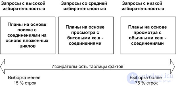
These three basic groups also allow the optimizer to determine the correct plans for such queries. The MS SQL Server optimizer is based on the main principle of query selectivity with respect to the fact table. A query is more selective the fewer rows from the fact table it uses. The percentages of rows retrieved from the fact table are used to create query classes. These percentages reflect values from typical customer queries, but are not strict boundaries for defining access paths.

The first class includes highly selective queries that process up to 15% of the fact table's rows. The second class, with medium selectivity, contains queries that process between 15 and 75% of the fact table's rows. Queries in the third class, with low selectivity, require processing more than 75% of the fact table's rows. The rectangles in the figure show the basic execution plans for each selectivity class.

Choosing a plan based on selectivity

Since highly selective queries against a star schema typically retrieve no more than 10-15% of the fact table's rows, they can be allowed random access to the table. Therefore, query plans for this class are based on nested-loop joins together with (nonclustered) index seeks and bookmark lookups on the fact table. Since these perform random I/O against the fact table, sequential I/O becomes more efficient when retrieving large amounts of fact table data. Therefore, as the number of rows retrieved from the fact table grows beyond a certain threshold, a different query plan is used.

Since medium-selectivity queries against a star schema process a significant fraction of the fact table's rows, access to the fact table typically uses hash joins with a fact table scan, or a range scan of the fact table. MS SQL Server uses bitmap filters to improve the performance of hash joins.

The join implementation for each join is a hash join, which allows MS SQL Server to take information about the matching rows from the dimension tables and obtain information about the join-reduction in cardinality for both dimension tables. The physical data access operator (for example, a table scan) uses this information about dimension table rows to eliminate fact table rows that do not satisfy the join conditions against the dimensions.

The optimizer removes these fact table rows as early as possible in query processing. This saves CPU time and can reduce disk I/O, because the removed rows do not need to be processed by later operators in the query plan.

The query optimization pipeline for star schemas

The optimization process uses standard query optimization heuristics to build an initial set of candidate execution plans. Special extensions are then invoked to produce additional plan variants.

In the case of data warehousing, the extension identifies star schemas, snowflake schemas, and star query sequences, and evaluates the query's selectivity with respect to the fact table. If the schema and the shape of the query match these sequences, the optimizer automatically adds the resulting query plans to the plan space, which is then analyzed by cost-based optimization to select the best plan for execution.

During query execution, MS SQL Server monitors the actual selectivity of join reduction as it runs. If the selectivity changes, MS SQL Server dynamically reorders the join-reduction information data structures so that the most selective one is applied first.

Star schema join heuristics

Most physical data warehouse models use a star schema but do not fully specify the relationships between dimension and fact tables, for example, through foreign key constraints. If foreign key constraints are not explicitly defined, the query optimizer must determine star schema query sequences using heuristics. The following heuristics are used for this.

• The largest of the tables participating in an n-ary join is considered the fact table. There are additional constraints on the minimum size of the fact table. For example, if even the largest table is smaller than a certain size, the n-ary join is not considered a star join.
• All join conditions of the binary relationships of a star query must be column equality predicates. The joins must be inner joins. This may seem restrictive, but it covers most joins between the fact table and dimension tables on surrogate keys in typical star schemas. If a join has more complex conditions that do not fit the pattern described above, it is excluded from the star join. For example, a five-way join could be reduced to a three-way join (with two additional joins applied later) if two of the joins have more complex predicates.

Note that these are heuristic rules. In practice, there are few situations in which the heuristic confuses the fact table with a dimension table. This affects the choice of plan but does not change the correctness of the chosen plan. The binary joins involved in a star query are then sorted in descending order of selectivity. Join selectivity in this context is defined as the ratio of the fact table's input cardinality to the resulting join cardinality, that is, join selectivity shows how much a given dimension reduces the fact table's cardinality. In general, joins with higher selectivity should be considered first.

The MS SQL Server query processor automatically applies this optimization to queries that match the star schema and the conditions mentioned above, when the resulting query plans are judged to be beneficial. Therefore there is no need to modify your application in order to take advantage of this way of improving performance.

Partitioned table parallelism

To speed up query processing in large data warehouses, administrators often partition large fact tables by date. The data is split into filegroups, reducing the volume of data that needs to be scanned when processing rows within a given range; it also allows the performance of the underlying disk system to be used simultaneously, when the filegroups are located on multiple physical disks.

As discussed in previous lectures, partitioning is successfully used to improve query processing, especially in large decision-support applications.

MS SQL Server 2008 includes a new feature — Partitioned Table Parallelism (PTP), which improves query performance in the case of partitioning by making better use of the available hardware's computing power, regardless of how many partitions a query touches or the relative size of individual partitions. In a typical data warehouse scenario with a partitioned fact table, users will notice a significant improvement for queries executed in parallel, especially if the number of available processor cores exceeds the number of partitions touched by the query. And this new feature works right away, without any additional configuration or changes.

Data compression

As business intelligence grows in popularity, enterprises add more and more data for analysis to their data warehouses. The result is exponential growth in the volume of managed data. The size of a data warehouse triples every two years. This raises new questions about managing such large data volumes and ensuring acceptable query performance against the warehouse. Such queries are typically complex, involving many joins and aggregates, and require access to large amounts of data. Moreover, many queries in the workload are I/O-bound.

Built-in data compression helps address this problem. MS SQL Server 2005 SP2 introduced a new variable-length storage format called vardecimal for decimal and numeric data. This new storage format can significantly reduce database size. The resulting reduction in size can, in turn, improve the performance of I/O-bound queries in two ways. First, fewer pages need to be read; and second, since the data is stored compressed in the buffer pool, the expected page lifetime increases (in other words, the probability that the needed page is already in the buffer increases). Of course, the space savings from data compression come at the cost of additional CPU load during compression and decompression.

SQL Server 2008 uses the vardecimal storage format, providing two kinds of compression: ROW compression and PAGE compression. ROW compression extends the vardecimal storage format by storing all fixed-length data types in a variable-length storage format.

Some examples of fixed-length data types are integer, char, and other rigid data types. Even though MS SQL Server stores these data types in a variable-length format, their semantics do not change (from the application's point of view, the data type remains fixed-length). This means you can take advantage of data compression without modifying your applications.

PAGE compression reduces data redundancy across columns in one or more rows on a given page. It uses a proprietary implementation of the LZ78 (Lempel-Ziv) algorithm, storing redundant data once per page and referencing it from multiple columns thereafter. Note that if you enable PAGE compression, ROW compression is used as well.

ROW and PAGE compression can be enabled for a table, an index, or one or more partitions of partitioned tables and indexes. This gives full flexibility in choosing which tables, indexes, and partitions to compress, allowing you to balance the space savings against the CPU overhead.

Partition-aligned indexed views

In SQL Server 2008, partition-aligned indexed views make it possible to build and manage shared aggregates in a relational data warehouse more efficiently, and to use them in scenarios where this was previously inefficient. This improves query performance. In a typical case, there is a fact table partitioned by date. Indexed views (or shared aggregates) are defined on this table to speed up queries. When a new partition is switched into the table, the corresponding partitions of the partition-aligned indexed views defined on the partitioned table are switched automatically as well.

The partition-aligned indexed views feature provides the benefits of indexed views on large partitioned tables without the need to rebuild aggregates over the entire partitioned table. These benefits include automatic maintenance of aggregates and indexed view matching.

Partition-level lock escalation

DBMSs in the MS SQL Server family support range partitioning, which lets you partition data for ease of management or group data according to usage patterns. For example, sales data can be partitioned by month or quarter. A partition can be mapped to its own filegroup, and a filegroup, in turn, to a group of files. This provides two advantages. First, you can back up and restore a partition as an independent unit. Second, you can map a filegroup to a fast or slow I/O subsystem, depending on the usage pattern or query load.

The data access pattern is an important consideration. Queries and DML operations may only need to access or manipulate part of the partitions. So, for example, if you are analyzing sales data for 2008, you only need access to the relevant partitions; ideally, queries accessing data in other partitions should have no effect on you at all (aside from shared system resources). In MS SQL Server 2005, concurrent access to different partitions sometimes resulted in table-level locking, which could impede access to other partitions.

To remove these limitations, SQL Server 2008 introduced a table-level setting that lets you control lock escalation at the partition or table level. The lock escalation policy for a table can be changed. For example, you can set lock escalation as follows:

ALTER TABLE  set (LOCK_ESCALATION = AUTO)

This command instructs SQL Server to choose a lock escalation granularity appropriate for the table's structure. If the table is not partitioned, lock escalation will occur at the TABLE level. If it is partitioned, the lock escalation granularity will be at the partition level. This setting is also used in SQL Server as a way to reduce the likelihood of table-level lock granularity.

Summary

In this lecture we discussed how relational DBMS query optimizers work. In particular, we presented a brief overview of features in the MS SQL Server 2008 family of DBMSs that help you achieve better performance for decision-support queries in relational data warehouses.

We covered a general procedure, important for a data warehouse designer, for tuning a SELECT command whose execution results do not meet performance requirements. This procedure is one iteration on the way to building an optimal set of indexes and consists of seven steps.

• Step 1. Update statistics.
• Step 2. Simplify the SELECT command.
• Remove unnecessary predicates and clauses.
• Add parentheses in arithmetic and logical expressions.
• Convert bound variables to constants.
• Step 3. Review the query plan.
• Converting a subquery into a join.
• When temporary tables will be created.
• Slow join methods.
• Step 4. Localize bottlenecks.
• Step 5. Create single-column indexes for critical parameters.
• Step 6. Create multi-column indexes.
• Step 7. Drop all indexes that are not used in the query plan.

Продолжение:

Часть 1 Tuning the performance of data warehouse queries
Часть 2 Analyzing queries to improve their execution speed - Tuning the