
Lecture
The simplest systems have a linear, unbranched structure. More complex
systems are organized by means of hierarchical structures. Alongside these two types of system organization, another type of structure is widespread, characterized by
an abundance of horizontal (single-level) connections. Such systems are known
as networks. The simplest system is a graph.
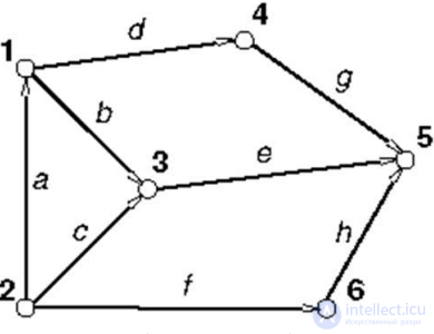
Fig. 4.1. Example of a directed graph
A graph G(V,E) is a system consisting of two sets: vertices (Vertices) and the edges (Edges) connecting them. A vertex and an edge are called incident if the vertex is one of the endpoints of the edge. Two vertices connected by
an edge are called adjacent. Edges sharing a common vertex are also called adjacent. A finite sequence of adjacent edges is called a route. A route in which all edges are different is called a chain. A chain in which
all vertices are different is called a simple chain. A graph G is called
connected if any two of its vertices can be joined by at least one chain. A chain whose starting and ending vertices coincide is called
a cycle. A connected graph having no cycles is called a tree. For any graph, a tree can be constructed that contains all of its vertices. Such a tree is called spanning, or a covering of the graph. If every edge of the graph has a direction, the graph is called directed (a digraph). A directed edge is called an arc. A network is a digraph in which every arc has a definite numerical
value (weight).
A graph can be specified by means of a drawing or by a list of vertices and edges. However,
the most convenient way of specifying a graph for computer processing
is by means of matrices. Consider the graph shown in Fig. 4.1. It can be specified by means of the following incidence matrix
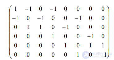
Each row of this matrix corresponds to a vertex, and each column to an arc. In each
column of such a matrix there is one 1 (entry), one –1 (exit), and the remaining elements are equal to zero.
Modeling the structure of systems by means of graphs makes it possible to solve many applied problems. Let us demonstrate the capabilities of graphs and networks in the field of
transport network optimization. A similar approach can be used for
analyzing computer network traffic, organizing construction work, and so on.
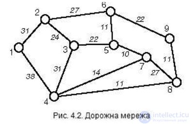
Suppose we are given a road network consisting of nine vertices (inhabited points) connected by edges (roads) as shown in Fig.2. It is necessary to find the shortest path from vertex 1 to vertex 8.
One of the methods for solving this problem is Dijkstra's algorithm. The algorithm
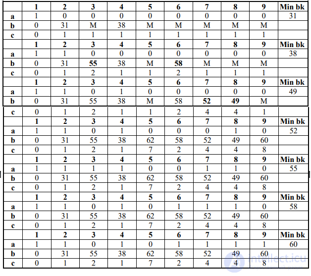
for this problem uses three arrays of n (n – the number of vertices) numbers each.
The first array a contains labels with two values: 0 (the vertex has not yet been examined) and 1 (the vertex has already been examined).
The second array b contains distances – the running shortest distances from the starting vertex Vi to another vertex Vk.
The third array contains vertex numbers – the k-th element ck is the number of the second-to-last vertex on the running shortest path from Vi to Vk. The distance matrix Dik gives the lengths of the edges dik; if no such edge exists, dik is assigned the value of a very large number M, equal to "machine infinity".
The algorithm for finding shortest paths in a network was first described by Dijkstra (1959). It consists of three steps and has the form:
1. Initialization. To all elements of array a except ai (the start of the route), assign
the value 0. ai := 1. To all elements of array b, assign the distance values from its row of the matrix Dik. To all elements of array c (except ci), assign the value i
(the number of the starting vertex). ci:=0.
2. Main part. Find the smallest distance bj among the unmarked columns
(i.e., for those j for which a[j]=0). Set a[j]:=1 (mark the vertex).
Consider all routes running from the vertex and through vertex j to vertex k.
Calculate their length bk. If bk > bj + djk (the length of the new route is less
than the length of the old one), then we set bk:=bj+djk; ck:=j. If bk < bj + djk (the new
route is longer than the old one) – no changes are made to the k-th column.
The main part is repeated until only one zero remains in array a.
The solution process can be represented in the form of the following tables.
3. Output. The length of the shortest path from vertex Vi
to vertex Vk equals bk. Now the vertices comprising the shortest path from Vi to Vk must be listed.
Array c serves this purpose. The last vertex is Vk, preceded by the vertex numbered ck, before which comes the vertex whose number is found in the
array c at position ck, and so on.
To execute the algorithm, array b of n elements must be scanned n times, i.e., Dijkstra's algorithm has quadratic complexity.
There are several cities that need to be connected by a network of roads. For each pair
of cities, the projected cost of building the connecting road is known. The task is to build the cheapest possible road network. Similar problems can be formulated for
water-supply or gas-pipeline networks.
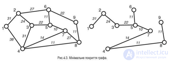
If we regard the road network as a graph, and consider the construction cost to be
proportional to the length of the edge connecting the corresponding vertices, we arrive
at the problem of constructing a graph of minimal length. A graph of minimal length
is always a tree, because if the graph contained a cycle, one of the
edges of the cycle could be removed without breaking the graph's connectivity. So we need to construct a
spanning tree of minimal length. The solution is given by the Prim
– Kruskal algorithm (a greedy algorithm).
1. We select the not-yet-considered edge of minimal length.
2. We attach it to the previously selected edges, provided that no cycle is formed.
3. After all edges have been examined, a spanning tree is formed, which will be the tree of minimal length.
The total length of the spanning tree is 134 km.
Closely related to the problem considered above is Prim's problem.
There are N inhabited points given by Cartesian coordinates on a plane (xi, yi).
The distance between the points is determined by the formula
 ( 4.1 )
The cost of building a road is considered proportional to its distance Dij. It is necessary to build a road network of minimal cost.
The solution algorithm is as follows.
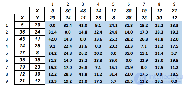
1. We construct the distance matrix using formula (4.1).
2. Using the Prim-Kruskal algorithm, we construct the minimum spanning tree.
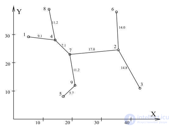
Fig.4.4. The shortest road network with a total length of 154 km.
An important application of the systems analysis of spatial networks is location problems.
When solving the problem of incorporating a new facility into an existing system of similar facilities, it is necessary to resolve the question of redistributing
the facilities' spheres of influence at minimal cost to the existing system.
Classic examples of facility-location problems on a network are the problems of school location and fire-station location.
A road network connecting
nine inhabited points is given (Fig.4.2). The number of pupils in the inhabited points is known
and equals: 20, 40, 60, 80, 10, 30, 50, 70, 90. It is necessary to choose the optimal location for the new school.
The solution is based on the following reasoning: the total distance
traveled by all pupils on their way to school must be minimal.
A theorem has been proved which states that the school must be located at one of the inhabited points.
First of all, it is necessary to construct the shortest-distance matrix, i.e., a matrix containing the lengths of the shortest chains connecting all points of the network with one another.
For this purpose, the Floyd algorithm is used, based on the triangle operation:
if d[i, k] + d[k,j] < d[i,j] then d[i,j]:=d[i,k]+d[k,j].
This operation replaces route [i j] with route [i k j] if it is shorter.
Floyd's algorithm.

The matrix d[i,j] is initialized as follows. If vertices i and j are directly connected, d[i, j] equals the distance between the vertices; otherwise, d[i, j] equals
M (machine infinity). After the algorithm finishes running, the matrix d[i,j] contains the desired values of the shortest-chain lengths.
For small networks, the shortest routes between vertices can be determined manually by choosing among the options.
Let us calculate the shortest-route matrix for the network shown in Fig. 4.2.
Table 4.1. The School Location Problem.
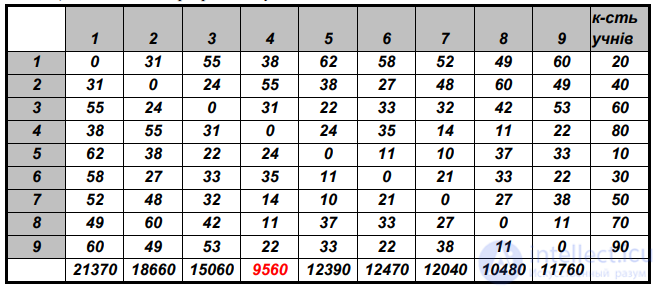
To the resulting matrix let us add one more column, containing the number of pupils pj in the inhabited points.
Let us also add an additional row containing sums of the form
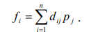 ( 4.2 )
The smallest of these sums (the fourth inhabited point) indicates the optimal location for the new school
Since formula (4.2) minimizes a sum, the school-location problem is called a minisum problem.
It is necessary to locate a responding fire station (a protection unit) that is called out to one of the points of the network (Fig. 4.2).
The main goal is: to reach the most distant point in the minimum possible time.
There are two options for solving the problem:
a) the fire station is at an inhabited point;
b) the fire station is outside an inhabited point. Let us consider only the first option.
Table 4.2. The Fire Station Location Problem.
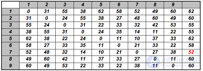
First we construct the shortest-route matrix. To the right of the matrix
we place a column in which we write down the largest of the numbers in the running row
(the distance to the most distant point). We find the smallest of these numbers. This will be the best option for locating the fire station. For our
problem this will be point 7. Since this algorithm finds the minimum among the maximum distances, the fire-station location problem
is called a minimax problem.
The algorithm for solving the problem when the fire station is located outside an inhabited point is considerably more complex.
The problem of locating the fire station outside an inhabited point.
Let us now consider the second option for solving the problem: locating the fire station outside an inhabited point.
First it is necessary to determine which of the network's edges are the most promising for locating the fire station (by performing a lower-bound estimate of the edges' distance from the farthest vertex).
Lower-bound estimate of an edge's distance from the farthest vertex.
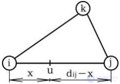
Fig.4.5. Locating the fire station on a network edge
Consider an edge (ij) connecting vertices i and j, as well as some other vertex k (Fig. 4.5). Let x be the coordinate (the distance from vertex i) of the fire station u on edge (ij).
The distance from vertex j to the fire station equals dij –x (dij – the length of edge (ij)). The optimal route from u to k is determined from the condition duk = min (x+dik, dij-x+djk).
The lower-bound estimate of the most distant point is determined from the condition
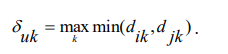 . (4.3)
Consequently, we must examine all vertices k  i,j. For each of them it is necessary to determine the value
  and then select the largest of them.
This will be the lower-bound estimate of the most distant point in the case where the fire station is located on edge (i,j).
This operation must be repeated for all edges, and the smallest of all the lower-bound estimates must be selected.
This will be the edge on which it is most advantageous to locate the fire station.
To illustrate the considerations above, let us examine an example.
As the network, let us consider the very same network we discussed at the beginning of this section.
Using the shortest-distance matrix constructed above, let us build
a table of lower-bound estimates (Table 4.3).
Table 4.3
Table of lower-bound estimates of an edge's distance from the farthest vertex 
Let us show, for example, how the first estimate for edge (1,2) – the number 49 – was obtained.
We compare pairs of numbers, one of which belongs to the first, and the other to the second row of the shortest-distance matrix between the vertices of the graph, constructed by us
earlier. Pairs corresponding to the first and second
columns are not included in the comparison.
We find

The lower-bound estimates of all the network's edges were found in a similar way. Analysis of the table shows that the most promising edges for locating the fire
station are edges (1,4) and (2,6), whose lower-bound distance estimate equals 35 km.
Now it is necessary to analyze both edges for the feasibility of locating the fire station.
The final stage in solving the problem of locating the fire station on a network edge is determining the optimal coordinate for locating the fire station.
on the edge with the minimal lower-bound distance estimate.
This problem is solved by the Hakimi algorithm.
Let the fire station u be located on edge (i,j) at a distance x from vertex i (Fig. 4.6). Let us calculate the distances from the fire
station to all vertices of the network. In our case, the optimal locations for the fire station are edges (1,4) and (2,6). Let us analyze
the second case. The length of the edge is 27 km. Consequently, if the distance from vertex 2 to the fire station is x km, then the distance from vertex 6 to the fire
station is 27 – x km.
Let us denote dui – the minimum distance from the fire station to the i-th vertex.
Then, for example, the distance to the first vertex will be determined by the condition
du1 = min (x+d21, d26 –x+d61 ) = min (31+ x, 58+27–x) = min(31+x, 85-x).
Given that 0 <= x <= 27, we obtain du1 = 31 + x.
Similar reasoning must be carried out for all the other vertices of the network.
As a result of this analysis we obtain:
du2 = x;
du3 = min(24+x, 33+27-x) = 24+x;
du4 =min(55+x, 35+27-x) = 62 - x;
du5 = min (38+x, 11+27-x) = 38 – x;
du6 = 27-x;
du7 = min (48+ x, 21+27-x) = 48 – x;
du8 = min(60+x,25+27 – x) = 52 - x;
du9 = min (49+x,22+27-x) = 49 – x.
Let us plot the graphs of the lines du1 – du9.
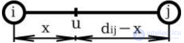
Fig. 4.6. Location of the fire station on edge (i,j)
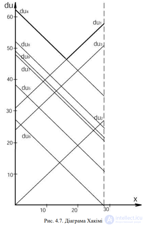
Fig. 4.7. The Hakimi Diagram
As a result we obtain the so-called
Hakimi diagram (Fig. 4.7). Its analysis shows that the optimal location of the fire station is the intersection point of lines du1 and du4. Let us solve the equation to determine the unknown coordinate x: 31 + x = 62 – x.
We obtain: x = 15.5; min dui=46.5 km.
A similar analysis carried out for edge (1,4) gives the result min dui = 52 km.
This means that this edge gives no gain compared with the previously chosen seventh inhabited point.
Conclusion. When locating the fire station at an inhabited point, the optimal option is the seventh inhabited point. In this case the distance to the most
distant point will be 52 kilometers. When locating the fire station outside an inhabited point, the optimal option is edge (2,6). The fire station should be located 15.5 km from point 2. In this case, the distance to the most distant point (the 1st or the 4th) will be 46.5 kilometers. Thus, compared with the first solution option, we obtain a gain of 5.5 kilometers. Locating the fire station on edge (1,4) gives no gain compared with locating it at inhabited point 7.
Remarks. It should be kept in mind that locating the fire station on an edge is not always more advantageous than locating it at a vertex of the graph. In each specific case, a conclusion can be drawn only after a complete analysis of both solution options. If several edges have the same minimal lower-bound distance estimate, the analysis using the Hakimi algorithm should be performed for all such edges.

Comments