
Lecture
System identification — a set of methods for building mathematical models of a dynamic system from observational data. In this context, a mathematical model means a mathematical description of the behavior of some system or process in the frequency or time domain — for example, physical processes (the motion of a mechanical system under the force of gravity), an economic process (the reaction of stock quotes to external disturbances), and so on. At present this area of control theory is well studied and finds wide application in practice.
The performance results of economic systems are reflected through the time series of their parameters. By examining the specifics of a time series, we can
draw conclusions about the nature of the system that generated it. In particular, based on the study of time series, conclusions are drawn regarding the dimensionality of the system,
the possibility of forecasting it and the maximum forecasting horizon, and the nature of the system's dynamics (trend-resistant, random, reversive). Therefore,
a mandatory stage preceding the modeling and forecasting of an economic system is the pre-forecast analysis of time series, which makes it possible to carry out
partial identification of the system. A mandatory element of system identification is determining the nature of its dynamics. The dynamics of a system can be deterministic (strictly defined, predictable) or random (stochastic, unpredictable). Some systems behave deterministically over certain time intervals
and randomly over other time intervals. A great deal
of information about the nature of a system's dynamics can be provided by the time series of values of one of the indicators characterizing the given system.
Let us consider methods for determining the degree of randomness of a system from its time series.
Consider a time series  in which every triple of consecutive values consists of distinct numbers. A turning point is a value of the series xt for which one of two conditions holds:
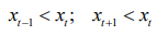 or
or 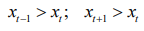 ;(M. Kendall).
Let us denote the minimum number from any triple of consecutive elements of the series  by the symbol a, the intermediate one – by the symbol b, and the maximum one – by the symbol c.
With a random arrangement of the numbers under consideration, 6 configurations are possible: a,b,c; a,c,b; b,a,c; b,c,a; c,a,b; c,b,a.
If the series is random, each of these configurations is equally probable, i.e., its probability of occurring in a random series is 1/6. Four of the six configurations listed above (all except the first and the last) correspond to the concept of a «turning point» as introduced by Kendall. The first and last configurations correspond to trend-like dynamics of the series. Thus, the probability of a turning point occurring in a
random series is 2/3, and the probability of a trend triad is 1/3. In this way M. Kendall showed that for a random (stochastic) series of length n
the average number of turning points is

with a standard deviation of

Let us introduce the following notation
 (7.1)
(7.1)
If the actual number of turning points Pf satisfies the relation 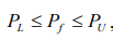 , the series is considered random (stochastic)
In a random series, as understood by Kendall, an increase (decrease) is followed by a decrease (increase) with probability 2/3, while the probability of yet another increase (decrease) is 1/3.
If the actual number of turning points Pf < PL, this means that the series is characterized by trend segments. Such a series is called persistent (trend-resistant).
If Pf > PU, this means an excessive number of fluctuations caused by some external factor. Such a series is called antipersistent (reversive).
Identifying a time series as trend-resistant or reversive is important for choosing a forecasting method. In the first case, extrapolation methods for trend models are used; in the second, harmonic or autoregressive models capable of reproducing the fluctuations of a random variable are used.
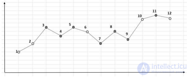
Fig. 7.1. Turning points (dark background)
A powerful tool for studying the nature of a system's dynamics is correlation analysis. By applying correlation analysis to the time series that
represents the system under study, one can obtain answers to the following questions: does the series have a trend? is there a cyclical component in the series? The first answer describes the direction of the system's dynamics (increasing, decreasing, stable),
while the second answer determines the presence (or absence) of fluctuations.
The correlational dependence between two different segments of a time series, shifted by a time interval L (lag), is called the autocorrelation with lag L.
The lag is the time interval between two segments of the time series.
Let us introduce the concept of the autocorrelation function (ACF)  for the time series
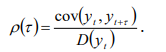 . (7.2)
Here  – is the covariance coefficient of the time series for lag
  ,
,
 – variance.
The value of the ACF characterizes the closeness of the statistical relationship between the levels of the time series separated by time lags.
All ACF values are dimensionless and satisfy the condition  . (7.3)
The graph of the ACF reflects the dependence of the autocorrelation coefficient on the lag and is called a correlogram.
When determining the number of ACF coefficients, the following rule is followed
 . (7.4)
Thus, the sequence of first-order, second-order, etc. autocorrelation coefficients forms the autocorrelation function of the time series. Analysis of the autocorrelation function and its graph (the correlogram) makes it possible to determine the lag at which the autocorrelation is highest, i.e., the lag at which the relationship between the current and previous levels of the series is closest.
Thus, by analyzing the autocorrelation function and the correlogram, one can identify the features of the dynamics of the system that generated the series. There are several rules describing the most characteristic examples of correlograms.
1. If the highest value is the positive first-order autocorrelation coefficient, the series under study contains only a trend (a tendency to increase or decrease).
2. If the highest value is the negative first-order autocorrelation coefficient, the series under study is reversive (prone to fluctuations).
3. If the highest value is the positive autocorrelation coefficient of order T, the series contains cyclical fluctuations with a periodicity of T.
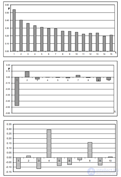
Fig. 7.2. Correlograms of a time series (TS).
A – a series with long memory (flooding of the Nile River);
B – a series with short memory (changes in winter wheat yield – USA);
C – a cyclical series (annual precipitation totals, Rivne region)
4. If none of the autocorrelation coefficients is statistically significant, we can assume that this series contains no trend or cyclical fluctuations and has a structure similar to that of a random process.
In practical studies, an autocorrelation coefficient is considered significant if its absolute value exceeds 0.2.
Let us consider several examples of correlograms constructed from real time series.
1. The ACF contains many significant elements. The series is prone to trends and has long memory (Fig. 7.2 A). The time series describes statistics on the magnitude of the flooding of the Nile (Egypt).
2. The ACF contains 1 significant element. The series is reversive and has short memory (Fig. 7.2 B). A series of winter wheat yields (USA).
3. Most of the ACF values are insignificant, but one of them is large and positive – evidence of a cycle with a period of 4 years (see Fig. 7.2 C). A series of annual precipitation totals for the Rivne region.
4. To construct a correlogram in MS Excel, the CORREL function can be used. For example, the function “CORREL($b$4 : $b$50; b5 : b51)” gives the value of the first autocorrelation coefficient
 for a series of 56 elements located in cells b4: b59; the function “CORREL($b$4: $b$50; b6 : b52)” ‒ gives the value of the second autocorrelation coefficient
  and so on.
However, the method described is not entirely accurate. Another method for constructing a correlogram is the Statistica program. In this case, the following sequence of commands is used: Statistics, Advanced Linear/Nonlinear Models, Time Series/Forecasting, Arima & autocorrelation functions, Number of lags, Autocorrelations.
The state of a system is characterized by the set of values of the system's main parameters
at a given moment in time. For example, to describe the economic state of an enterprise, one must specify numbers estimating gross output, income,
profit, profitability, number of employees, payroll fund, labor productivity, volumes of accounts payable and receivable, investment volumes, and equipment depreciation ratio. Let us denote these parameters by the symbols q1, q2 , q3 ,… qk .
These numbers are called the coordinates of the system’s state in the k-dimensional state space, or phase space.
When the state of a system changes, its parameters change, meaning the state coordinates are variable quantities that depend on time.

.
The most important characteristic of phase space is its dimensionality, i.e., the minimum number of parameters that must be specified to determine
the state of the system. The dimensionality of the phase space that provides an unambiguous representation of all possible states of the system is a numerical estimate of the system's complexity
.
Systems whose state changes over time are called dynamic. Each state of the system corresponds to a specific point in phase space

. The change of states of a dynamic system over time is called a process.
Any process in an economic system is characterized by a change in its parameters, and therefore corresponds to the motion of a point in phase space. The process of state change corresponds to a trajectory
– a line connecting neighboring points in phase space. The phase trajectory reflects the system's behavior under the influence of certain factors. The set of all phase trajectories corresponding to different initial conditions is called the phase portrait of the system. A phase portrait is a family of continuous curves. This means that a dynamic system can be in any given state
only once.
Most economic systems belong to the class of open nonlinear systems called dissipative systems. Such systems are non-equilibrium because of the dissipation of resources (matter, energy, money) obtained from outside. For such systems, the set of phase trajectories is attracted to a certain finite-dimensional subset of phase space called an attractor. A finite-dimensional attractor determines the properties of the oscillating process that becomes established in the system over time. Fluctuations in economic systems are non-periodic and are caused by overproduction crises, imperfections in financial mechanisms, the lack of equivalence between the mass of goods and the money supply, overproduction or underproduction of food, military and political conflicts, and so on. Some dynamic systems are characterized by a strange attractor (Fig. 7.4). This means that small changes in a system's initial conditions can lead to drastic changes after some time. A butterfly flapping its wings in one place on the globe can cause a hurricane in another place (B. Mandelbrot – the butterfly effect).
Changes in state parameters are described by functions that are either continuous or discrete.
When these functions are continuous, the behavior of the dynamic system is described using a system of differential equations:
 . (7.5)
Three characteristic types of behavior, or three modes, in which a dynamic system can be found are distinguished: equilibrium, periodic, and transient. Equilibrium of a system is its ability to maintain its state indefinitely (both in the absence and in the presence of external influences). According to the second law of thermodynamics, in the absence of control actions, a complex isolated system tends
toward a state of equilibrium characterized by disorganization and chaos.
In a cyclic mode of operation, the system returns to the same state after certain intervals of time (it arrives at the same point in phase space). Cyclicality is a form of stability. Examples: the cyclicality of seasonal product manufacturing, the cyclicality of transportation.
The process by which a system transitions from one stable state to another is called a transient process. A change in an object's state is inevitably associated with the transfer of matter, energy, or finances, and cannot occur instantaneously. The speed of the transient process characterizes the system's inertia. Transient processes are described using a logistic function.
A linear approach does not allow one to analyze the irregular behavior exhibited by modern financial markets. Until the early 1960s, only periodic and quasi-periodic motions had been observed in the steady-state regime of nonlinear dissipative dynamic systems. However, in 1963, Lorenz discovered a very complex motion in a dynamic system that was perceived as chaotic. To describe the properties of such motions, the concept of «dynamic chaos» was introduced. The word «dynamic» means that there are no sources of fluctuations. The word «chaos» means that the system's behavior can be predicted only for a very short interval of time. The Lorenz system describes the process of convection in a layer of fluid between two horizontal plates whose temperature is constant, with the lower plate being hotter than the upper one by ∆T. Experimental study of the situation for various values of ∆T showed that, at small temperature differences, the fluid is at rest and
only the mechanism of thermal conductivity operates, with the temperature falling linearly from the bottom to the surface. Then, upon reaching a certain critical temperature difference ∆Tc
the state becomes unstable. Hexagonal cells appear on the surface of the fluid, or convective rolls form. As ∆T increases further, the rolls begin to oscillate,
then the oscillations become increasingly complex and turbulent motion develops (Fig. 7.3).
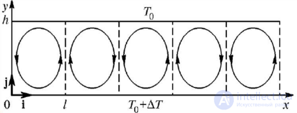
Fig. 7.3. Turbulent motion in the Lorenz system.
In a paper by the mathematicians Ruelle and Takens, published in 1971, a new mathematical image of dynamic chaos was introduced – the strange attractor. The word
"strange" emphasizes two properties of the attractor. First, its
geometric structure is unusual. The dimension of a strange attractor is fractional (fractal). Second, the strange attractor is a region that attracts trajectories from neighboring regions. At the same time, all trajectories inside the strange attractor are dynamically unstable, which is expressed as a strong (exponential) divergence
of trajectories that are close at the initial moment.
The mathematical model of the Lorenz system has the form:
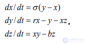 . (7.6)
Here the variable x depends on temperature, while the variables y and z depend on the projections of the fluid's velocity in the horizontal and vertical directions. A flat projection of the phase portrait of the Lorenz system is shown in Fig. 7.4.
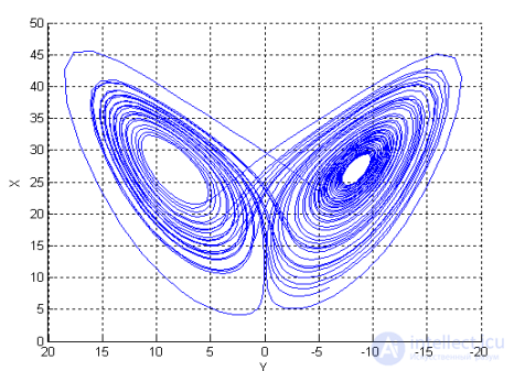
Fig. 7.4. Phase portrait of the Lorenz system (two-dimensional projection)
The phase portrait consists of two groups of cyclic trajectories located in two different planes positioned at an angle to one another. The transition of the trajectory from one plane to the other occurs randomly and unpredictably. This is precisely what constitutes the chaotic nature of the system. A sign of its dynamism is the almost periodic repetition of the trajectory's loops.
The simplest type of dynamic system behavior is linear dynamics, characterized by a uniform increase or decrease of the characteristic
indicator. More complex is periodic dynamics, characterized by regular periods of growth and decline of the indicator. Periodic dynamics is characteristic of nonlinear systems. The most complex type of dynamics is chaotic dynamics. Here the system's parameters likewise have regular periods of growth and decline, but the duration and amplitude of the fluctuations are variable. Over short time intervals, systems with chaotic dynamics are deterministic, but the forecasting horizon of such systems is always limited, since
their behavior depends strongly on the initial conditions. For systems with chaotic dynamics, it is possible to construct models using differential (difference) equations. To establish the type of dynamics characteristic of the system under study, a number of methods have been developed, most of which are based on the analysis of time series. Most time series are non-stationary, so at the first stage of the study it is necessary to model and remove the trend and the cyclical component from the series. The series obtained after this is called the residual series. If the trend of the time series is complex in nature and cannot be extracted using standard methods (elementary functions), the residual series may contain a deterministic component associated with that trend. To extract the deterministic component from the residual series, the residual series must be smoothed. Studying the smoothed residual series makes it possible to construct
the phase portrait of the system; to calculate the dimensionality of the system; and to assess the degree of its predictability.
Constructing the phase portrait. The use of chaotic dynamics methods requires the length of the series under study to be 102 – 103 elements. If the series under study are shorter, the ergodic hypothesis is used, and one long series is modeled by a set of shorter series for which the property of homogeneity holds (stability of the mean and variance). For example, when studying the dynamics of grain yields, the length of the time series is 60 elements. However, the presence of cycles of approximately equal duration makes it possible to treat each series as several loops of the phase trajectory. Such series contain three cycles (three loops of the phase trajectory) with an average duration of 19 years. Then, by considering a group of 12 regions with homogeneous yield dynamics, we obtain 36 loops of the phase trajectory with a length of 19 years. According to the ergodic principle, such a set of time series can be regarded as the analogue of a single time series with a length of 684 elements.
The shape of a dynamic system's attractor determines the nature of the system's dynamics. An attractor in the form of a point corresponds to a stable, stationary state. of the system (the system's settings do not change). An attractor in the form of a closed curve describes regular cyclic fluctuations of the system. A strange attractor describes complex, non-periodic fluctuations of the system. An important task is the reconstruction of the system's attractor from time series data. According to Takens-Mañé theory, a satisfactory geometric picture of the system's attractor can be obtained if, instead of the variables characterizing the system's behavior (whose values are unknown to us), one uses so-called
delay vectors  for a single measured parameter.
This approach to time series analysis was first mathematically justified in the works of Takens. Takens' theory makes it possible to establish the dynamic nature of a system.
To study the dynamic characteristics of a system, it is necessary to perform an
embedding of the system into phase space. For this, the method of time delays (lags) is used.
A D-dimensional phase space is constructed using a single time series 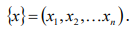
. For a lag value of L = 1, the first column vector has the form 
, the second column has the form 
, and the last column has the form 
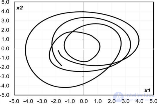
Fig. 7.5. Two-dimensional projection of the phase portrait of Ukraine's grain production system
Two segments of a time series, shifted relative to each other by some lag  , can be regarded as different parameters x1 and x2.
Let us consider the plane  , whose coordinates are the elements of the series X1 and X2
. The graph of the dependence  forms the phase trajectory of the system. D segments of the time series, shifted by a lag
  , form a D-dimensional model (reconstruction) of the system’s phase portrait.
Before constructing a phase portrait from real time series, they must be smoothed. Fig. 7.5 shows a two-dimensional projection of the phase portrait of Ukraine’s grain production system, obtained from a set of smoothed residual series. The behavior of the system’s phase trajectory shows pronounced cyclicality.
To analyze a system, one must first establish its dimensionality, i.e., the minimum number of parameters needed to describe the system. A small value of the dimensionality indicates that the system is deterministic, while a large value indicates that it is random. For dimensionalities not exceeding 5 – 6, a variety of methods for analyzing and forecasting the evolution of the system work well. Usually the explicit form of the system's mathematical model is unknown, and therefore it is necessary to be able to estimate the system's dimensionality directly from observations. The "false nearest neighbors" method and the eigenvalue method are used to determine the dimensionality. The false nearest neighbors method uses the concept of proximity of phase vectors. To determine the distance between vectors
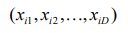 and
and  the Euclidean definition of distance is used
 . (7.7)
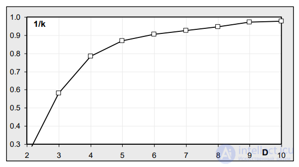
Fig. 7.6. Determining the minimum embedding dimension D
As the dimensionality of phase space D increases, the appearance of new nonzero coordinates causes an increase in the distance between two points. of the space – the phase-space stretching effect. The procedure for estimating the system's dimensionality begins with dimension 2. A group of phase-space vectors with the smallest distance between them is selected – the ”nearest neighbors”. The dimensionality is then increased by 1, and the coefficient k of the increase in distance between the vectors – the ”nearest neighbors” – is calculated. The dimensionality of the system is chosen as the number D
such that, when moving to dimension D +1, the distance between the ”nearest neighbors” increases only slightly (less than 10%). For example, Fig. 7.6 shows that for D > 4
the growth of the distance between ”neighbor vectors” is insignificant. Therefore the embedding dimension of Ukraine's grain production
system can be estimated at 4.
To implement the method, we first reduce the series to a zero mean, i.e., we make the substitution
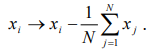 . (7.8)
We then form an observation matrix M from the resulting series according to the following rule:
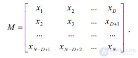 . (7.9)
The rows of this matrix contain the components of the vectors reconstructed from the time series.
We will choose the reconstruction dimension ( D = 8 ) deliberately larger than the expected dimensionality of the system. Based on the matrix M
we form the covariance matrix
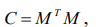 , (7.10)
and calculate its eigenvalues 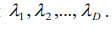
. The eigenvalue calculations can be performed in Matlab using the eig(C) function, which returns the vector of eigenvalues of the square matrix C.
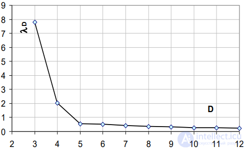
Fig. 7.7. Determining the embedding dimension using the eigenvalue method
As a rule, the first few eigenvalues will be noticeably larger than the others, which are roughly equal to one another. At a certain eigenvalue number, the eigenvalue magnitudes stabilize (reach a plateau). This number is then the dimensionality of the system. The results of calculations using the eigenvalue method are shown in Fig. 7.7. As the figure shows,
for D >5 the eigenvalue magnitudes stabilize.
Consequently, D = 5 is the dimensionality value of the system under study.
Determining the maximum Lyapunov exponent. A fundamental characteristic of a dynamic system is the set of Lyapunov exponents, which describe
the behavior of trajectories in phase space. Lyapunov exponents are denoted by the symbols  and can be negative, positive, or zero. The number of Lyapunov exponents equals the dimensionality of the system. Each exponent reflects the average rate of divergence (
  ) or convergence (
  ) of initially close phase trajectories in a given plane.
The value of the maximum Lyapunov exponent makes it possible to identify the type of the system's dynamics:
 < 0 the system evolves toward a state of equilibrium,
for  = 0 the system’s dynamics are cyclical,
in the case where  > 0 , the system’s dynamics are chaotic.
Knowledge of the system’s maximum Lyapunov exponent is very important, since it determines the extent to which the system’s development can be forecast.
First, in two of these cases the system is predictable, and we can forecast its development for an arbitrarily long period of time. When chaotic dynamics
are present in the system, the maximum forecasting time is limited due to the rapid divergence of phase trajectories. The value of the maximum forecast horizon
Tmax is determined from the relation Tmax =1/λmax
. For example, for Ukraine’s grain production system, λmax= 0.05, and the maximum forecasting horizon is Tmax= 20 years.

Comments