
Lecture
To determine the state of a system, one needs to evaluate (measure) the values of its main characteristics. Measurements underlie systems analysis. Let us denote
by 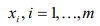 the observed properties of the system, and by
 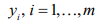 – the notation for these properties.
The set of symbols used to record the states of an object is called a measurement scale. Measurement scales differ in their strength depending on the operations they permit. The weakest are nominal scales, and the strongest are absolute scales.
Three main attributes of measurement scales are distinguished:
1. ordering of data means that one point of the scale is greater or less than another point;
2. interval property of scale points means that the interval between one pair of numbers is greater or less than the interval between another pair of numbers;
3. zero point (reference point) means that the scale has a reference point corresponding to the complete absence of the property being measured.
All scales are divided into two groups:
- qualitative (non-metric) scales, which lack units of measurement (nominal and ordinal scales);
- quantitative (metric) scales – interval scale, ratio scale, and absolute scale.
The scale of names (nominal scale) is a finite set of designations for
different states of an object. In this case, the main attributes of measurement
scales are absent, namely ordering, interval property, and zero point. Measurement consists in determining an object's membership in one state or another and recording
this with a symbol denoting that state. This is the simplest scale,
used only to distinguish one object from another.
Examples:
- geographic names, personal names of people, etc.;
- car license plate numbers, official document numbers, numbers on athletes' jerseys.
The need for classification also arises in cases where the classified states form a continuous set. The entire set is divided into several subsets, which are denoted by certain symbols. Example. At a mathematics olympiad, 5 participants shared first place, the next 5 participants shared second
place, and so on. When processing data on a nominal scale, only the operation of checking their coincidence or non-coincidence can be performed with the data.
Next in strength after the nominal scale is the ordinal scale. This scale has ordering, but lacks the attributes of interval property and zero point.
Measurement on an ordinal scale can be applied in the following situations:
- when it is necessary to order objects in time or space.
- when it is necessary to order objects according to some quality.
Between the values of an ordinal scale there exist the following types of relations: a) equality
or inequality of values; b) the "greater than" or "less than" relation between different values of variables.
The ordinal scale is used in evaluating gymnasts' performances and figure skating scoring.
But here one cannot say that an athlete who received 10 points performed twice as well as one who received 5 points.
Typical types of ordinal scales
By denoting classes with symbols and establishing order relations between these symbols, we obtain a simple order scale. Examples: prize places in competitions ("gold", "silver", "bronze"), social status ("poor", "middle class", "elite").
A variant of the ordinary order scale is opposition scales. They are formed from pairs of antonyms located at opposite ends of the scale (strong-weak,
warm-cold).
Sometimes it turns out that certain pairs cannot be ordered and are considered equal: A ≥ B and B ≤ A, i.e., A = B. The corresponding scale is called a weak-order
scale
Example: kinship relations (mother = father > son = daughter, uncle = aunt < brother = sister, etc.).
If there are objects in the set that cannot be compared with each other, i.e., neither A ≥
B nor B ≤ A holds, then this is called a partial-order scale. For example, a person may be unable to assess which of two products he prefers (a mobile phone or a music player); which type of favorite activity
(football or listening to music).
Modified ordinal scales
Sometimes reinforcing modifications of the ordinal scale are used.
Examples:
1. The hardness scale. In 1811, the German mineralogist F. Mohs proposed
establishing a hardness scale by introducing ten gradations. The following
minerals were adopted as standards, in increasing order of hardness: 1 – talc, 2 – gypsum, 3 – calcite, 4 – fluorite, 5 –
apatite, 6 – orthoclase, 7 – quartz, 8 – topaz, 9 – corundum, 10 – diamond. Of two minerals,
the harder one is the one that leaves scratches or dents on the other upon sufficiently
forceful contact. However, the gradation numbers of diamond and apatite do not give grounds
to claim that diamond is twice as hard as apatite.
2. The Beaufort wind force scale. In 1806, F. Beaufort proposed
a conventional 12-point scale for assessing wind force based on its effect on objects on land and on sea waves:
3. The Richter magnitude scale for earthquakes. The American seismologist
Richter proposed a 12-point earthquake scale in 1935, based on magnitudes
based on assessing the energy of seismic waves that arise during earthquakes.
4. Grading scales for assessing students' knowledge. 5-point, 100-point.
Next in strength is the interval scale, which, unlike the previous ones, is a quantitative scale. The interval scale has ordering and
interval properties, but no zero point. On the interval scale, only the intervals
have the meaning of real numbers, and arithmetic operations can be performed on them. The values themselves are not true numbers, and the results of operations on them
may be meaningless. For example, it is incorrect to state that the temperature
of water increased twofold when heated from 10°C to 20°C.
The following property holds for the interval scale:
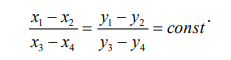 . (2.1)
For the interval scale, the starting point can be chosen arbitrarily, for example, for temperature or terrain elevation.
Temperature, time, terrain elevation – quantities which, by their physical nature, either have no absolute zero or allow freedom of choice in establishing the starting point.
Example 1 – temperatures (Celsius scale and Kelvin scale).
Let us heat water from 10°C to 20°C on the Celsius scale. On the Kelvin scale this corresponds to temperatures from 283 0K to 293 0K. On both scales the temperature difference
is the same – 10.
Example 2 – calendars.
A person's lifespan is the same in all calendars.
Periodic scales
A special case of interval scales is periodic scales. On such a scale, the value does not change when a certain number (the period) is added. Examples: a compass
scale, a clock face.
Ratio scale
Next in strength is the ratio scale. For measurements on this scale,
any arithmetic operations can be performed. This scale has all the attributes:
ordering, interval property, zero point.
Examples of ratio scales: weight, length, money. Comparing two objects,
we can see how many times the property of one object exceeds the same property of the other object.
An absolute (metric) scale has both an absolute zero (b=0) and an absolute unit (a=1).
Examples: 1. The number line OX; 2. The Kelvin temperature scale.
When taking measurements, one often encounters the concept of uncertainty. One type of uncertainty is randomness. Randomness is a type of uncertainty that obeys only a probability distribution law. Knowing the probability distribution
p(x), one can answer most questions about a random variable: which interval its possible values belong to; around which value they are scattered
(the sample mean); how widely these values are dispersed (variance or standard deviation), and so on. Usually it is sufficient to know not the entire distribution, but only some of its parameters (sample mean, variance).
Another type of uncertainty is fuzziness of data. Fuzziness situations most often occur when using linguistic constructions.
Indeed, in the expression "a tall young man" – the class to which the person belongs is named, but it is not known how tall he is or how old he is. Other examples: "hot", "cheap", "smart".
A linguistic variable is a variable whose value is inherently vague. A mathematical apparatus has been created for operations with linguistic variables
– fuzzy set theory. To establish an object's membership in a fuzzy
set, the concept of a membership function is used 
. For each
element x one can assign a number 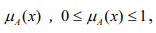 , which expresses the degree to which this element belongs to the fuzzy set A.
If  , then element x does not belong to set A; if
  ‒ it belongs.
A fuzzy set A is denoted as a collection of ordered pairs of the form
 . (2.2)
Example 1: "the student studies well" {(2,0.0); (3,0.2); (4,0.8); (5,1.0)}.
Example 2: "a warm day" {(15,0.4); (20,0.7); (25,1.0); (30,0.4); (35,0.1)}.
High dimensionality. In many studies, the number of objects N and the number of their features n are large, so the product N x n has several orders of magnitude.
Accounting for time leads to an even greater increase in the dimensionality of the data block N x n x t. The use of computers substantially expands data-processing capabilities,
but the "curse of dimensionality" remains a serious problem.
Various techniques are used to reduce the dimensionality of a model. For example, there are the following economic indicators: GDP, budget deficit, external
debt, inflation rate, monetization ratio, dollarization ratio. If several features correlate
with one another, only one of them is retained, and the others are discarded. Another approach is factor analysis. Several new artificial factors are introduced that do not correlate with one another and fully reflect the influence of all the input data.
Heterogeneity of data. Different features are measured on different scales and in different units.
Most algorithms are designed to process variables of the same type, so it is necessary to reduce the data to a single scale and dimensionality, or to build an algorithm for processing heterogeneous data. The classical approach is standardization of features.
For each feature x, the mean value xc and standard deviation 
are determined.
Standardization is performed according to the relation
 . (2.3)
As a result of standardization, all variables become dimensionless, and their numerical values lie in the range from –2 to +2.
Missing values. Unfilled cells in a data table are often encountered. The simplest way to recover a missing value is to compute
the average between the preceding and following values.
Noisiness. Measurement results usually differ from the actual values by some random quantity – error. If the statistical properties of the error do not depend on the quantity being measured, the error is called additive noise. Signal filtering is used to remove noise.

Comments