
Lecture
Risk-aware optimization of systems — is an approach aimed at improving the operation of complex systems while taking into account possible risks and uncertainties. The main goal is to find a balance between system efficiency and risk management in order to minimize losses or possible negative consequences. This process can include several steps:
Risk identification: Determining possible risk factors (external and internal) that can affect the system. This can include financial, technical, environmental and other types of risks.
Assessment of probabilities and consequences: For each risk, its probability and possible consequences for the system are determined. Probabilistic methods and data analysis are applied here.
Defining optimization criteria: It is necessary to establish objective functions for optimization, which include both minimizing risks and maximizing system performance.
Development of models and methods: Various mathematical and statistical methods are applied, such as linear and nonlinear programming methods, stochastic models, Monte Carlo methods and others.
Monitoring and control: After the optimized solution is implemented, continuous monitoring is carried out to assess how the system copes with risks in practice.
This approach can be applied in various fields, such as:
In risk-aware asset portfolio management, the main task is to find the optimal ratio between return and risk. This allows investors to minimize possible losses while maintaining an acceptable level of return. The process includes the following key stages:
Various metrics are used to manage risk in a financial portfolio:
It is important to establish the desired return based on investment goals. In the portfolio management process, it should be kept in mind that higher returns are often associated with increased risks.
Based on the given levels of risk and return, various optimization methods are applied:
Markowitz model (Mean-Variance): This classical portfolio optimization model involves finding a portfolio with minimal volatility for a given level of return. It is based on calculating the covariances between assets to construct an efficient frontier, which determines the portfolios with the best return-to-risk ratio.
Sharpe model: This model uses the Sharpe ratio, which measures a portfolio's risk-adjusted return, to select the optimal portfolio. The higher the Sharpe ratio, the better the portfolio compensates for risk.
Optimization with regard to VaR and CVaR: More complex optimization models can take into account not only volatility but also possible extreme losses. This is especially useful under unstable market conditions.
Robust methods: To account for uncertainties in parameters (for example, in the volatility or correlations of assets), robust optimization can be used, which creates portfolios resistant to changes in market conditions.
Diversification is a key risk-management tool. It is important to distribute assets across different classes (stocks, bonds, commodities, etc.) and regions in order to reduce the overall risk of the portfolio. This reduces the likelihood that a negative event in one area will strongly affect the entire portfolio.
After an optimized portfolio has been formed, it is necessary to regularly monitor its performance and adjust its structure depending on changes in market conditions, as well as changes in the investor's risk preferences.
If an investor is willing to accept a moderate level of risk, a diversified portfolio can be created that includes stocks with low Beta and high-quality bonds. Using CVaR will help avoid significant losses during periods of market instability.
Risk-aware optimization of an asset portfolio helps investors make more informed decisions, taking into account their risk tolerance and market conditions.
In the energy sector, managing power grids with regard to risks and possible failures is a key task for ensuring reliable and efficient supply to consumers. Modern power systems are becoming increasingly complex due to the integration of renewable energy sources, which increases uncertainty and the likelihood of failures. Risk-aware optimization of such systems helps reduce the likelihood of disruptions and minimize the consequences in the event of failures.
This method involves integrating risk assessment at the design and planning stage of power grids. It includes forecasting possible failures and determining measures to prevent them.
These models take into account uncertainties such as weather conditions and unpredictable consumption. Stochastic optimization helps find solutions that are resilient to various scenarios of how events may unfold.
When a system is close to overload or a failure occurs at one of its nodes, it is important to properly distribute loads to minimize damage. In such cases, energy distribution optimization is applied:
Robust optimization models are developed to account for uncertainties and maintain system stability even under changing parameters. For example, they can account for sharp changes in energy production from renewable sources.
Incorporating distributed energy resources (such as solar panels, wind turbines, batteries) can increase the reliability of power grids. Decentralized energy production reduces dependence on large generators and can be used as a reserve in the event of failures.
Collecting data from various parts of the grid (using sensors and IoT devices) makes it possible to predict and prevent possible equipment failures. This helps not only reduce repair costs but also improve the overall reliability of the system.
Given the growing number of cyberattacks on power systems, protecting data and networks plays an important role. Reliable mechanisms for detecting and preventing cyber threats can prevent outages and disruptions.
In the event of disruptions, restoration systems play a key role in minimizing downtime. Optimizing restoration plans involves determining priorities for restoring critical grid elements.
Suppose a power grid uses energy from both renewable and traditional generators. To account for the risk of failures associated with wind farms, a model can be developed that includes stochastic forecasting of wind speed and load distribution. If the wind is insufficient, the system can automatically switch to other sources, using optimization methods to minimize costs and ensure stability.
Risk-aware optimization of power grid management is aimed at increasing their resilience and reliability. Methods including data analysis, failure modeling and load forecasting help minimize the impact of disruptions on consumers and ensure the stability of power systems.
Risk management in production processes is a critically important task for ensuring uninterrupted operation, safety and product quality. Modern enterprises face numerous risks that can affect production efficiency, costs and company reputation. These risks can include technical failures, non-compliance with safety standards, market changes, or supply chain disruptions.
Risk management begins with identifying and assessing risks. It is necessary to identify potential risks at all stages of the production process, from raw material procurement to finished product release.
Stochastic modeling is used to assess the probability of risks and their consequences. This helps forecast potential disruptions and develop a response strategy.
One of the risk-management methods is optimizing production processes aimed at increasing their resilience to disruptions.
Automating processes and introducing digital technologies reduce the risk of human error and increase the accuracy of operations.
Using predictive technologies to prevent equipment breakdowns before they lead to serious disruptions is becoming an important risk-management tool.
To minimize risks associated with supplies, it is important to have supply chain management strategies.
Given the increasing reliance on information technology, especially with the use of IoT and digital control systems, it is critically important to protect production systems from cyberattacks.
Effective risk management requires continuous monitoring of production processes and real-time data analysis.
A manufacturing company that depends on a complex supply chain can use digital twins to model its processes. With predictive maintenance, it can prevent equipment breakdowns, and with data analysis, it can identify the most vulnerable points in the supply chain. Automating management using SCADA systems allows tracking equipment status in real time, reducing the risk of unplanned downtime.
Risk management in production processes improves the reliability and efficiency of an enterprise's operation, minimizes costs and increases safety. Optimizing processes, introducing predictive technologies and automation can significantly reduce the impact of potential risks on production.
System optimization – is a set of methods that allow choosing, from among many possible options for using resources, the one that is best from the standpoint of
achieving the economic result with the lowest costs.
Let us demonstrate the optimization methodology using the example of economic systems.
Every economic system pursues the goal of its own functioning. Most often – this is
obtaining maximum profit or minimum costs. There exists some function F, which describes the degree to which the goal is achieved and is expressed in terms of the input variables and
the parameters of the system:
 (8.1)
(8.1)
Here xj (j=1,2,...,n) are the controllable variables, which can be managed; yi (i=1,2, ..., m) are
the uncontrollable variables, whose values are determined by the external environment;
c1 ,c2 , ,ci ...— are the parameters of the system, which are fixed.
For example, sown area – is a controllable variable, while air temperature – is an uncontrollable variable; the qualitative composition of the soil – is a system parameter.
In general terms, the problem of economic-mathematical modeling is formulated as follows:
Find the following values of the controllable variables xj , for which the objective function F
takes on its maximum or minimum value:
 . (8.2)
The objective function F determines the efficiency of the system's functioning.
The possibilities for choosing xj are always limited by external conditions. For example, the sown area is limited by the availability of arable land and other resources. These processes
can be described by a system of mathematical inequalities (or equations) of the form:
 (8.3a)
or
 (8.3b)
System (8.3a) – (8.3b) is called the system of constraints of the problem. For economic systems, the variables xj
must be nonnegative:
 . (8.4)
Relations (8.2) – (8.4) form the economic-mathematical model of the linear programming problem for the economic system.
Any set of variables x1, x2, ..., xn, satisfying conditions (8.3) and (8.4),
is called a feasible plan. Each feasible plan determines a certain strategy of behavior for the economic system. Each feasible plan corresponds to
a value of the objective function, calculated using formula (8.2).
The set of all solutions of the constraint system (8.3) and (8.4) forms the region of feasible plans.
The plan for which the objective function takes on an extreme value is called optimal. The optimal plan is the solution of the linear programming problem (8.2) – (8.4).
The solution of a linear programming problem is sought using the simplex method. This method is implemented in the Excel package – Data, Solver.
Economic systems exist under conditions of uncertainty. This means that we do not know what state the system will be in at a future moment in time. Uncertainty always gives rise to risk. This can be the risk of lost profit, the risk of losses, the risk of unused opportunities, etc.
Decision-making under uncertainty is characterized by the fact that it is impossible to unambiguously foresee its consequences. As a result, profit becomes a random or fuzzy quantity, which can be maximized only by taking into account the probability of various scenarios of how events may unfold, the degree of certainty of various features, and the risk tolerance of the decision-maker.
The causes of uncertainty and the risk resulting from it are divided into three groups.
The first group. Most economically related processes are random. It is difficult to foresee various natural phenomena, climate changes, political events,
changes in world market conditions, the emergence of new technologies, changes in consumer tastes, and so on.
The second group. One can speak of an economically optimal incompleteness of
information, because it is often more expedient to work with incomplete information than to
collect very expensive, virtually complete information. Incompleteness of information can
also be due to its incomplete understanding or the inability to process it on a
computer. In addition, any information is always inexact (statistics, sample observations, expert assessments).
The third group. There is the so-called asymmetry of information. Major players in the economic market consider it expedient to conceal a certain part of the information from consumers for economic, political or other reasons.
The role of information in the decision-making process is extremely great.
Relevant (truthful, important) information available to a narrow circle of persons is especially valuable. After such information is published, the broad mass of entrepreneurs uses it to make business decisions, and this information quickly loses its value. A lack of information (uncertainty) always gives rise to risk. One has to deal with risk in everyday practical activity.
It cannot be avoided in any type of business activity. Risk is present when deciding on placing money in a bank, when buying stocks and other securities, when investing funds in new production, and so on.
Inaction in the sphere of business is associated with the risk of unused opportunities. Note that risk exists only when there are different possible scenarios of how events may unfold.
There are different approaches to defining risk. According to V. Marshall's definition, risk – is the probability of an adverse event occurring. E. J. Henley and H. Kumamoto regard risk as the probability of material damage or harm. Risk is often understood not only as the possibility of damage occurring, but also as
the possibility of deviation from the goal, the absence of expected results.
Generalizing, one can say that risk – is a recognized danger
of the occurrence of events with undesirable consequences. Risk – is a quantitative value and is determined by multiplying the probability of a negative event by the magnitude of the possible damage from it.
In the 1960s, such fields of science as the theory of random processes, fuzzy set theory, game theory, and statistical decision
theory developed. These scientific disciplines made it possible to optimize the management of economic systems taking into account the uncertainty and risk inherent in them.
Most investors usually invest in several objects of the real or financial sector, forming a set of assets (an investment portfolio)
The portfolio approach involves maximizing the utility of the assets, i.e. increasing their return through diversification (variety) for the purpose of
reducing investment risks. Reducing risk through a combination of assets implements the principle expressed by the proverb «don't put all your eggs in one basket» (the probability of dropping two baskets is significantly lower than the probability of dropping one). Thus, a compromise is achieved between such seemingly incompatible goals as maximizing income and minimizing risk.
Nobel laureate Harry Markowitz was the first to point out that when forming a securities portfolio, one must take into account not only their return but also their degree of risk. The main parameters of the Markowitz model are the return
and riskiness of the securities included in the portfolio. The Markowitz model is based on the following assumptions:
The return of a securities portfolio – is the weighted average return
of the securities included in the portfolio, determined by the formula:
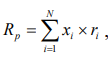 , (8.5)
where:
N ‒ is the number of securities included in the portfolio;
xi ‒ is the percentage share of the given security in the portfolio ( );
);
ri ‒ is the return of the given security.
The return of a given type of stock ri over a minimal time interval (1 day or 1 week) is usually calculated using the ratio
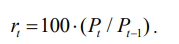 . (8.6)
Here Pt-1 — is the stock price at the previous moment in time,
Pt – is the stock price at the next moment in time.
For long-term observations, the return of a security is estimated as the average value over the observation period
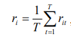 , (8.7)
where
T – is the number of time intervals.
The risk of financial operations directly depends on the variability of external conditions
and the value of securities. The greater this variability, the greater the risk of financial operations.
In the Markowitz model, the risk of a security is regarded as the standard deviation of its return from its mathematical expectation.
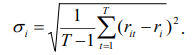 . (8.8)
To assess portfolio risk, it is necessary to take into account both the risks of individual stocks and correlation risks. The latter are related to the fact that losses can increase if stock
prices behave in a correlated manner and can fall simultaneously. The correlation coefficient between two securities is calculated using the formula
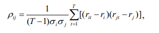 , (8.9)
where:
 — the return of securities i and j in period t
. Then the overall risk of the securities portfolio  is determined by the standard deviation function:
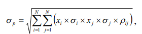 , (8.10)
where:
ixi , xj ‒ the percentage share of the given securities in the portfolio;
 , ‒ the risks of the given securities (standard deviations);
 ‒ the linear correlation coefficient between the returns r it and r jt .
It is impossible to simultaneously achieve maximum income and minimum risk. Therefore the problem is solved in stages: one parameter is constrained and the other is optimized. Thus, two approaches to solving the portfolio investment optimization problem are considered. The first (the direct Markowitz problem) consists in imposing a certain constraint on the degree of risk – the risk must not
exceed a certain permissible level 
. The return of the portfolio in this case must be maximal. The mathematical description of the Markowitz model for the problem of maximizing return will look as follows:
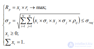 (8.11)
Here
ix – is the relative share of the i-th asset in the bank's portfolio,
ir – is the return, calculated as the average return over the period under study,
 is the risk of the i-th asset, calculated as its standard deviation over the period under study,
 - the maximum permissible risk value, set by an expert,
 – the linear correlation coefficient between the returns of two types of assets. Problem (8.11) is nonlinear and cannot be solved using the simplex method.
To solve such problems, nonlinear programming methods are used, in particular the capabilities of Microsoft Excel (Solver).
The second approach to solving the Markowitz problem (the inverse Markowitz problem) consists in minimizing risk while maintaining a certain guaranteed
level of return. The mathematical description of the Markowitz model for the problem of minimizing risk will look as follows:
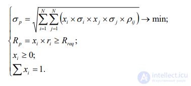 (8.12)
Example 1. As shown above, when forming a securities portfolio, the principle of diversification should be observed. According to this principle, securities that are not correlated with one another, or better still, that have a negative correlation, are included in the portfolio. Let us consider a portfolio consisting of two types of stocks. The portfolio's rate of return is calculated using the formula
 . (8.13)
Here
i x – is the share of the i-th security in the portfolio structure;
i r – is the expected profit value of the i-th type of stock.
For non-stationary behavior of the stock price, the expected profit value is often estimated as the slope of the stock price trend
over a certain base segment.
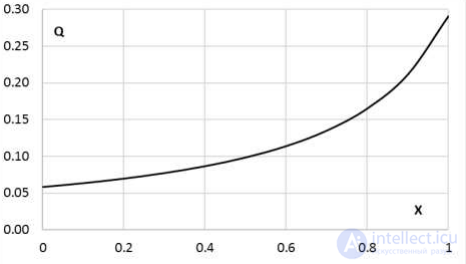
Fig. 8.1. Dependence of the monetary attractiveness Q of a pair of stocks on its composition x.
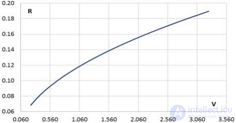
Fig. 8.2. Dependence of return R on risk V for a pair of stocks
The risk of a two-stock portfolio is determined by the formula
 . (8.14)
Here
 - is the standard deviation of the price of the i-th type of stock;
 - is the correlation coefficient of the two stocks.
The financial attractiveness Q of a pair of stocks is estimated as the ratio of expected profit to portfolio risk
 . (8.15)
The task is to maximize the financial attractiveness of the pair of stocks.
The dependence of the monetary attractiveness of a pair of stocks on its composition is shown in Fig. 8.1.
The dependence of portfolio return on its risk is shown in Fig. 8.2.
As we can see, higher return is accompanied by greater risk.
This conclusion can be considered a general law of economics.
Example 2. The Markowitz model is applicable to the optimization of agricultural production. Let us consider an agricultural enterprise growing 3 crops: wheat, sugar beet and potatoes. Known statistics on the profitability of these crops over the last 10 years are available. The average profitability of the crops, respectively  , will be regarded as the profit
. The risk of each crop will be assessed through the standard deviation of the corresponding profitability 
The weighted average profitability of the three crops is calculated using the formula
 . (8.16)
Here
xi – is the share of the i-th crop in the total sown area;
ri – is the average profitability of the corresponding crop.
The risk of a three-crop portfolio is determined by the formula
 . (8.17)
Here
 - is the standard deviation of the profitability of the i-th crop;
 – is the correlation coefficient of the profitability of two crops.
The task is to maximize profit (weighted profitability) under a limited risk. The mathematical model for the formulated agricultural production problem will look as follows:
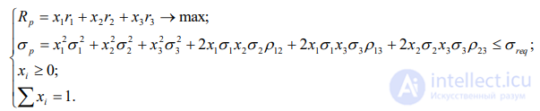 (8.18)
The dependence of the return of the three-crop portfolio on its risk is shown in Fig. 8.3. Again we see that the maximum value of return is associated with the maximum value of risk, and vice versa.
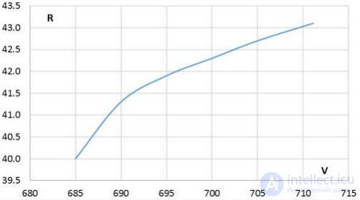
Fig. 8.3. Dependence of return R on risk V for a portfolio of three crops

Comments