
Lecture
System identification — a set of methods for building mathematical models of a dynamic system from observational data. In this context, a mathematical model means a mathematical description of the behavior of some system or process in the frequency or time domain — for example, physical processes (the motion of a mechanical system under the action of gravity), an economic process (the reaction of stock quotes to external disturbances), and so on. At present, this area of control theory is well studied and finds wide application in practice.
The beginning of system identification as a subject of building mathematical models from observations is associated with the work of Carl Friedrich Gauss «Theoria motus corporum coelestium in sectionibus conicis solem ambientium», in which he used the least squares method he developed to predict the trajectories of planetary motion. Subsequently, this method found application in many other areas, including the construction of mathematical models of controlled objects used in automation (motors, furnaces, various actuators). Most of the early work on system identification was done by specialists in statistics and econometrics (who were particularly interested in identification applications related to time series) and formed an area called statistical estimation. Statistical estimation was also based on the work of Gauss (1809) and Fisher (1912).
Until approximately the 1950s, most identification procedures in automatic control were based on observing the responses of controlled objects to certain control actions (most often actions of the following types: step (H⋅1(t)), harmonic (sin(α),exp(jω)), generated colored or white noise), and depending on what type of information about the object was used, identification methods were divided into frequency-domain and time-domain methods. The problem was that the application of these methods was mostly limited to scalar systems (SISO, Single-input, single-output). In 1960, Rudolf Kalman introduced the state-space description of a controlled system, which made it possible to work with multidimensional (MIMO, Many-input, many-output) systems as well, and laid the foundations for optimal filtering and optimal control based on this type of description.
Specifically for control problems, system identification methods were developed in 1965 in the works of Ho and Kalman , and Åström and Bohlin . These works paved the way for the development of two identification methods that remain popular to this day: the subspace method and the prediction error method. The first is based on the use of projections in Euclidean space, while the second is based on minimizing a criterion that depends on the model parameters.
The work of Ho and Kalman is devoted to finding a state-space model of the object under study having the lowest possible order of the state vector, based on information about the impulse response. This same problem, but now in the presence of realizations of a random process where a Markov model is formed, was solved in the 1970s in the works of Faurre and Akaike . These works laid the groundwork for the creation of the subspace method in the early 1990s.
The work of Åström and Bohlin, meanwhile, introduced the maximum likelihood method to the identification community — a method that had been developed by time-series specialists for estimating the parameters of models in the form of difference equations . These models, known in the statistical literature as ARMA (autoregressive moving average) and ARMAX (autoregressive moving average with exogenous input), later formed the basis for the creation of the prediction error method. In 1970, Box and Jenkins published a book that gave a significant boost to the application of identification methods in every field where this was possible. This work provided, put simply, a complete recipe for identification, from the start of data collection about the object to obtaining and validating the model. For 15 years, this book remained the main reference on system identification. Another important work of that time was a survey devoted to system identification and time-series analysis, published in IEEE Transactions on Automatic Control in December 1974. One of the open questions at the time was the identification of closed-loop systems, for which the cross-correlation-based method leads to unsatisfactory results[10]. From the mid-1970s onward, the newly invented prediction error method came to dominate both the theory and, more importantly, the applications of identification. Most of the research activity focused on problems of identifying multivariable and closed-loop systems. The key task for these two classes of systems was to find experimental conditions and ways of parameterizing the problem such that the resulting model would approach the one and only exact description of the real system. All of the activity of that period can be described as a search for the «true model», and as work on questions of identifiability, convergence to exact parameters, the statistical efficiency of estimates, and the asymptotic normality of the estimated parameters. By 1976, the first attempt was made to regard system identification as an approximation theory, in which the task is to find the best possible approximation of the real system within a given class of models[11][12],[13]. The prevailing view among identification specialists thus shifted from searching for a description of the true system to searching for a description of the best possible approximation. Another important breakthrough occurred when L. Ljung introduced the concepts of bias and variance error for estimating transfer functions of objects[14]. Work on bias and variance analysis of the resulting models during the 1980s led to the perspective of viewing identification as a synthesis problem. Based on an understanding of the influence of experimental conditions, model structure, and identification criterion — grounded in bias and error variance — it becomes possible to tune these design variables to the object so as to obtain the best model within a given class of models[15][16]. This ideology permeates the book by Lennart Ljung[17], which has had a great influence on the identification community.
The idea that model quality can be altered through the choice of design variables led to a surge of activity in the 1990s that continues to this day. The main application of this new paradigm is identification for model-based control. Accordingly, identification for control problems has developed extensively since its emergence, and the application of identification methods to control has breathed new life into already well-known research areas such as experiment design, closed-loop identification, frequency-domain identification, and robust control under uncertainty.
The main event in the development of system identification in the USSR was the establishment in 1968 of Laboratory No. 41 («Identification of Control Systems») at the Institute of Automation and Telemechanics (now the Institute of Control Sciences of the Russian Academy of Sciences), with the support of N. S. Raibman. Naum Semyonovich Raibman was one of the first in the country to recognize the practical value and theoretical interest of system identification. He developed the theory of dispersion identification for identifying nonlinear systems[18], and also wrote a book titled «What Is Identification?»[19] to explain the basic principles of the new subject and describe the range of problems addressed by system identification. Later, Yakov Zalmanovich Tsypkin also took an interest in identification theory, developing the theory of information identification[20]
Building a mathematical model requires 5 basic things:
 .
.Input-output information is usually recorded during a pre-planned identification experiment, during which the researcher can choose which signals to measure, when to measure them, and which input signals to use. The discipline of «Experiment Design» can suggest how to make the experimental information as informative as possible, given the constraints that may be imposed on the experiment. Unfortunately, however, it is not uncommon for the researcher to have no opportunity to conduct an experiment at all, and instead to work with whatever information has been provided.
The set of candidate models is obtained by deciding on the class of models within which the search will be conducted. Without a doubt, this choice is the most important and the most difficult part of the identification procedure. It is at this stage that all prior information and engineering intuition must be combined with the formal properties of the candidate models in order to make a decision. The set of candidate models can also be built on the basis of known physical laws, or it is possible to use standard linear models with no reliance on physics whatsoever. Models that are not built on known physical laws, and that have parameters which can be adjusted to bring them closer to the object under study, are called black-box models. Models that have adjustable parameters while relying on known physical laws are called gray boxes. Generally speaking, a model structure is a parameterized mapping from the set of inputs and outputs up to and including the time instant t−1 to the set of outputs at the current time instant t
 :
:

The criterion for choosing a model is its ability to reproduce the data obtained from the experiment, that is, to match the behavior of the object under study. It must be remembered, however, that a model can never be accepted as a «real» or «true» description of the object, owing to its inherent approximate nature.
It is possible to build a «white box» model based on first principles , for example, a model of a physical process based on Newton's equations , but in many cases such models will be too complex and, possibly, even impossible to obtain within a reasonable time, owing to the complex nature of many systems and processes.
Therefore, a more common approach is to start with measurements of the system's behavior and of the external influences (inputs to the system), and try to determine the mathematical relationship between them without going into detail about what is actually happening inside the system. This approach is called system identification. Two types of models are common in the field of system identification:
In the context of nonlinear system identification, Jin et al. [ 9 ] describe gray-box modeling as assuming a model structure a priori and then estimating the model parameters. Parameter estimation is relatively straightforward if the form of the model is known, but this is rarely the case. As an alternative, the structure or terms of the model — for both linear and very complex nonlinear models — can be identified using NARMAX methods . [ 10 ] This approach is fully flexible and can be used with gray-box models, where the algorithms are populated with known terms, or with fully black-box models, where the model terms are selected as part of the identification procedure. A further advantage of this approach is that the algorithms will simply select linear terms if the system under study is linear, and nonlinear terms if the system is nonlinear, which provides greater flexibility in identification.
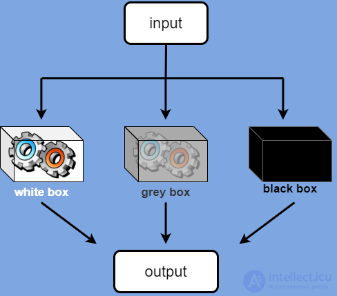
fig. A diagram describing various system identification methods. In the «white box» case we clearly see the structure of the system, while in the «black box» case we know nothing about it except how it reacts to input data. The intermediate state is the «gray box» state, in which our knowledge of the system's structure is incomplete.
The identification procedure has a natural logical order: first we collect data, then we form a set of models, and then we choose the best model. It is a common occurrence for the first model chosen to fail the test of matching the experimental data. In that case, one should go back and choose a different model or change the search criteria. A model may be unsatisfactory for the following reasons:
Identification assumes the experimental study and comparison of input and output processes, and the task of identification consists in choosing an appropriate mathematical model. The model must be such that its response and the response of the object to one and the same input signal are, in a certain sense, close to each other. The results of solving the identification problem serve as initial data for the design of control systems, optimization, analysis of system parameters, and so on.
At present, the following methods are used to determine the dynamic properties of controlled objects:
Static mathematical models of systems are obtained in three ways: experimental-statistical, deterministic, and mixed.
Experimental-statistical methods require conducting active or passive experiments on the operating object. Stochastic models are used to solve various problems related to the study and control of processes. In most cases, these models are obtained in the form of linear regression equations.
Given the properties of real processes, it can be argued that the equations relating the process variables should have a different, possibly more complex, structure. The further the structure of the regression equations is from the «true» one, the lower the prediction accuracy will be as the range of variation of the process variables increases. This degrades the quality of control and, consequently, reduces the quality of the object's operation in the optimal regime.
Deterministic models are constructed «on the basis of physical laws and conceptions of the processes involved». Consequently, they can be obtained even at the process design stage. At present, several methods for building mathematical models of continuous processes have been developed on the basis of the deterministic approach. For example, the method of multidimensional phase space is used in the mathematical modeling of a number of processes in chemical technology. The essence of the method is that the course of the modeled technological process is treated as the motion of certain «representative points» in a multidimensional phase space. This space is defined as the space of a Cartesian coordinate system, along whose axes are laid out the spatial coordinates of the apparatus and the internal coordinates of the reacting solid particles. Each point in the multidimensional phase space describes a specific state of the modeled process. The number of these points equals the number of particles in the apparatus. The course of the technological process is characterized by the change in the flow of representative points.
The method of multidimensional phase space is the most widely used for building mathematical models . However, this method also has drawbacks that limit its range of application:
Thus, because of the features of the multidimensional phase space method listed above, it is quite difficult to use it for building mathematical models of technological processes based on data obtained without conducting experiments on industrial facilities.
As a rule, theoretical analysis of a process makes it possible to obtain a mathematical model whose parameters need to be refined during the control of the technological object.
Despite the large number of publications on the parametric identification of dynamic objects, insufficient attention is paid to the identification of non-stationary parameters. When examining the known approaches to non-stationary parametric identification, two groups can be distinguished .
The first group includes works that make substantial use of prior information about the parameters being identified. The first approach in this group is based on the hypothesis that the identified parameters are solutions of known homogeneous systems of difference equations, or are represented as a random process generated by a Markov model, that is, are solutions of known systems of differential or difference equations with white-noise-type disturbances characterized by a Gaussian distribution with known mean values and intensity. This approach is justified when a large amount of prior information about the sought parameters is available, and if the real parameters do not correspond to the adopted model, it leads to a loss of algorithm convergence.
The second approach, also belonging to the first group, is based on parameterizing the non-stationary parameters and uses the hypothesis that non-stationary identified parameters can be represented exactly, over the entire identification interval or over individual sub-intervals, in the form of a finite, usually linear, combination of known functions of time with unknown constant weighting coefficients — in particular, as a finite sum of terms of a Taylor series, a harmonic Fourier series, or a generalized Fourier series in systems of orthogonal Laguerre or Walsh functions.
The simplest case of parameterization is the representation of non-stationary parameters as constant values over a sequence of individual sub-intervals covering the identification interval.
For current identification, it is recommended to switch to a sliding time interval [t — T, t] of duration T and to treat the sought parameters as constant over this interval, or as exactly representable in the form of a finite-degree interpolation polynomial, or the aforementioned finite linear combination. Works based on the use of the iterative least squares method can be assigned to this approach. In these works, owing to the use of an exponential (with a negative exponent) weighting factor in the minimized quadratic functional defined on the current time interval [0, t], old information about the object's coordinates is gradually «erased» over time. This situation essentially corresponds to the idea of constancy of the identified parameters over a certain sliding time interval, while taking into account information about the state of the object over this interval with an exponential weight.
This approach makes it possible to directly extend methods for identifying stationary parameters to the case of identifying non-stationary parameters. In practice, however, the underlying hypothesis of this approach does not hold, and one can speak only of an approximate representation (approximation) of the sought parameters by a finite linear combination of known functions of time with unknown constant weighting coefficients. This situation gives rise to a methodological identification error, which fundamentally changes the essence of the approach under discussion, since the duration T of the approximation interval and the number of terms in the linear combination become regularization parameters. This methodological error is, as a rule, not taken into account. In particular, under the assumption of a rectilinear law of variation of the sought parameters over sub-intervals significantly longer than T, and given a number of constraints on the statistical characteristics of the coordinates of the object's regression model and of the acting noise, an adaptive algorithm for correcting the parameter T was proposed. Neglecting the methodological error means that the approach under consideration turns out to be, in essence, completely unexplored; the region in which it works under non-stationary identified parameters is undefined, and this approach can be said to be applicable only in the particular case where the stated hypothesis holds exactly.
The second group includes methods that use a significantly smaller amount of information about the sought parameters, with this information being used only at the stage of choosing the parameters of the identification algorithm.
The first approach in this group is based on the use of gradient self-tuning models. This approach has been discussed in works on the parametric identification of linear and nonlinear dynamic objects. The main advantage of this approach is that it leads to a closed-loop identification system and thus offers certain advantages in terms of noise immunity compared with open-loop identification methods. The drawbacks of this approach are related to the need to measure components of the gradient of the tuning criterion, which are functional derivatives; the requirement for sufficiently accurate prior information about the initial values of the identified parameters (in order to choose initial model parameter values that guarantee the stability of the identification system's operation); and the lack of a complete theoretical analysis of the dynamics of this type of identification system. The latter is explained by the complexity of the system of integro-differential equations describing the processes in the self-tuning loop, as a result of which theoretical analysis is carried out only under the assumption of slow variation of the object's and model's parameters. Because of this, it is not possible to fully evaluate the region of stability, the speed, and the accuracy of gradient self-tuning models, and thus it is not possible to clearly define the range of applicability of systems of this type for the current identification of non-stationary parameters. As the degree of non-stationarity of the sought parameters increases, the methodological errors in determining the components of the gradient of the tuning criterion increase significantly, as a result of which the identification error grows beyond the region of the global extremum of the minimized criterion.
This effect is especially amplified as the number of identified parameters increases, owing to the interdependence of the identification channels. Therefore, the use of gradient self-tuning models is fundamentally limited to the case of slowly varying sought parameters.
The second approach is based on the use of the Kaczmarz algorithm. It is known that the basic algorithm of this type has weak noise immunity and low speed. This has prompted the creation of various modifications of this algorithm, characterized by increased speed. Nevertheless, the speed of these modifications remains low, which a priori limits the range of applicability of the second approach to the identification of slowly varying parameters.
The second group can also include methods intended for identifying only linear dynamic objects, which are characterized by additional constraints (the need to use test input signals in the form of a set of harmonics or a pseudo-random periodic binary signal, the finiteness of the identification interval, the availability of complete information about the object's input and output signals over the entire identification interval, and the possibility of identifying coefficients only for the left-hand side of the differential equation). Because of this, significant identification errors are possible over individual finite sub-intervals of time, and a complex boundary-value problem must also be solved.
In automatic control, the typical test input signals are:
A number of methods (representing parameters as solutions of known systems of differential or difference equations) can find application only in special cases, while other methods (gradient self-tuning models, the Kaczmarz algorithm) are a priori characterized by significant restrictions on the degree of non-stationarity of the sought parameters. The noted drawbacks arise from the very nature of the methods mentioned, and therefore there is hardly any possibility of noticeably reducing these drawbacks. Methods based on parameterizing non-stationary parameters, as noted above, are completely unexplored and, in their present form, may find only limited practical application. However, unlike the other methods, this last approach contains no internal restrictions on the degree of non-stationarity of the identified parameters and turns out to be, in principle, applicable to identification over long time intervals for a wide class of dynamic objects operating under normal conditions.
The difficulties listed above in identifying real operating systems determine the approach to modeling nonlinear objects that is most oriented toward widespread use — namely, choosing the type of mathematical model in the form of an evolution equation followed by parameter identification, or non-parametric model identification. A model is considered adequate if the estimate of a given adequacy criterion, computed as the dependence of the model's residual on the experimental data, falls within acceptable limits.

Comments