Robotic perception

Robotic perception is the process by which robots display the results of sensory measurements on the internal structures of the representation of the environment. The task of perception is complex, since the information coming from the sensors is usually noisy, and the environment is partially observable, unpredictable and often dynamic. As a rule of thumb, one can be guided by the fact that high-quality internal presentation structures have three properties: they contain enough information so that the robot can make the right decisions, are built so that they can be updated effectively, and are natural in the sense that internal variables correspond to the natural state variables in the physical world.

Models of transition and perception for a partially observable environment can be represented using Kalman filters, hidden Markov models, and dynamic Bayesian networks; in addition, in this chapter, both accurate and approximate algorithms for updating the confidence state — the distribution of a posteriori probabilities over environmental variables — were described. Several dynamic models of Bayesian networks were given for this process. And when solving robotic problems, the model usually includes the own past actions of the robot as observable variables. The figure shows the notation used in this chapter: x _t is the state of the environment (including the robot) at time t; z _t - observational results obtained at time t; A _t is the action taken after receiving these observation results.

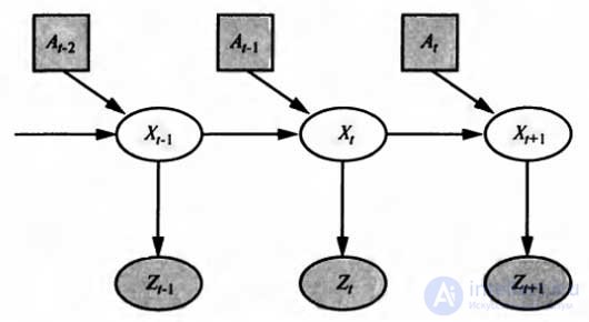
The process of robotic perception, considered as a temporary algorithmic conclusion based on sequences of actions and measurements, which is demonstrated by the example of a dynamic Bayesian network

The task of filtering or updating the trust state is that the new trust state P must be calculated (x _{t + 1} I z _{1: t + 1} , a _{1: t} ) based on the current trust state P (x _t I z _{1: t} , a _{1: t-1} ) and the new observation z _{t + 1} . The principal differences compared with this chapter are as follows: firstly, the results of the calculations are clearly not only due to the actions, but also to the observations, and, secondly, we now have to deal with continuous and not with discrete variables. Thus, it is necessary to correct the recursive filtering equation as follows in order to use integration in it, and not summation:

P (X _{t + 1} l IZ _{1: t + 1} l, a _{1: t} ) = aP (z _{t + 1} l X _{t + 1} ) ∫ P (X _{t + 1} , x _t. A _t ) P (x _t lz _{1: t} , a _{1: t-1} ) dx _t

This equation shows that the posterior probability distribution over state variables x at time t + 1 is calculated recursively based on the corresponding estimate obtained one time step earlier. These calculations involve data on the previous action at and current sensory measurements z _{t +1} . For example, if the goal is to develop a football-playing robot, then x _{t +1} can represent the location of the soccer ball relative to the robot. The distribution of the posterior probabilities P (X _t | z _{1: t} , a _{1: t -1} ) is the distribution of probabilities over all states, reflecting everything that is known about the past results of sensory measurements and control actions. The equation shows how to recursively evaluate this location, incrementally deploying the computation and including in this process sensory measurement data (for example, camera images) and robot motion control commands. The probability P (x _{t +1} | x _t , a _t ) is called a transition model , or a motion model , and the probability P (z _{t +1} I x _{t +1} ) is a perception model.