Configuration space

In robotics, decisions are ultimately embodied in the movements of the actuators. The task of the positioning movement is to deliver the robot or its final actuator to the specified target position. This is a difficult task, but even more difficult is the task of a matching motion , during which the robot moves while in physical contact with an obstacle. An example of a matching movement is the winding of a light bulb with a robot arm or a robot pushing a box to move it across a table surface.

We begin with the search for a suitable representation that would allow us to describe and solve problems of motion planning. As it turned out, more convenient for operation compared to the original three-dimensional space is the configuration space - the space of the robot states, determined by the position, orientation and rotation angles of the hinges. The task of planning a path is to find a path from one configuration to another in the configuration space. The main families of approaches used in this process are known as cell decomposition and skeletization . In each of these approaches, the task of planning a continuous path is reduced to the problem of searching in a discrete graph based on the identification of certain canonical states and paths in free space. Throughout this section, it is assumed that the movements are deterministic, and information about the localization of the robot is accurate. In the following sections, these assumptions will be weakened.

Configuration space

The first step to solving the robot motion control problem is to create a suitable representation of the problem. Let's start with a simple representation for a simple task. Consider the robot arm shown in figure a) . It has two hinges that move independently of each other. As a result of the movement of the hinges, the coordinates (x, y) of the elbow and the grip change (the manipulator cannot move in the z direction). This description shows that the configuration of this robot can be described using four-dimensional coordinates: use the coordinates (x _e , y _e ) to indicate the location of the elbow relative to the medium and the coordinates (x _g , y _g ) to indicate the location of the capture. Obviously, these four coordinates fully characterize the state of the robot. They constitute a representation, which is commonly referred to as the workspace representation, since the coordinates of the robot are specified in the same coordinate system as the objects that it must manipulate (or which collisions should avoid). The workspace views are well suited for collision testing, especially if the robot and all objects are represented using simple polygonal models.

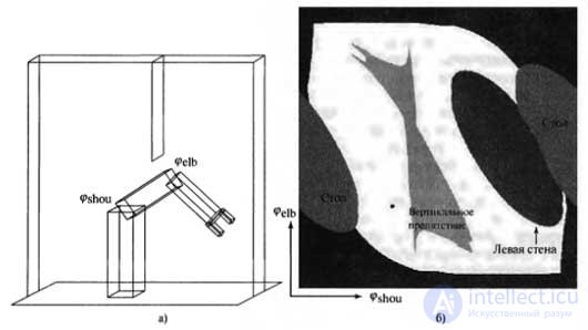
Comparison of presentation methods: representation of the working space of a robot manipulator with two degrees of freedom; the workspace is a box with a flat obstacle in the form of a plate hanging from the ceiling (a); configuration space of the same robot. In this space, only areas marked in white correspond to configurations in which collisions with obstacles do not occur. The dot in this figure corresponds to the configuration of the robot shown on the left (b)

But the working space view has one drawback due to the fact that not all work space coordinates are achievable, even in the absence of obstacles. This is due to the presence of constraints of communication in the space of reachable coordinates of the working space. For example, the position of the elbow (x _e , y _e ) and the position of the grip (x _g , y _g ) are always separated by a constant distance, since the hinges corresponding to these positions are connected with a rigid forearm. The robot scheduler with an algorithm defined on the coordinates of the working space faces the problem of developing such paths that allow you to adhere to these restrictions. Such a task becomes especially difficult due to the fact that the state space is continuous and the constraints are non-linear.

As it turned out, it is easier to plan based on the configuration space representation. Instead of representing the state of the robot using the Cartesian coordinates of its elements, this state is represented using the configuration of the hinges of the robot. In this example, the design of the robot includes two hinges. Therefore, its state can be represented by two angles, φ _s and φ _e , relating respectively to the hinge of the shoulder and to the hinge of the elbow. In the absence of any obstacles, the robot can freely choose any value from the configuration space. In particular, when planning a path, you can link the current and target configuration with a straight line. In this case, following this path, the robot can simply change the angles of rotation of its hinges at a constant speed until the target location is reached.

Unfortunately, the configuration space-based approach has its drawbacks. The task for the robot is usually expressed in the coordinates of the workspace, and not in the coordinates of the configuration space. For example, it may be necessary for the robot to place its final actuator at a specific coordinate in the workspace, possibly also indicating its orientation. In this regard, the question arises: how to map such coordinates of the workspace to the configuration space? Generally speaking, the inverse problem is easier to solve — the transformation of the coordinates of the configuration space into the coordinates of the working space, since it suffices to perform a series of quite obvious coordinate transformations. These transformations are linear for prismatic hinges and trigonometric for rotary hinges. Such a chain of coordinate transformations is called kinematics .

The inverse problem of calculating the configuration of a robot for which the actuator is located in the coordinates of the working space is called inverse kinematics . The problem of calculating inverse kinematics is usually difficult, especially for robots with many degrees of freedom. In particular, this solution is rarely unique. For the robot manipulator considered as an example, there are two different configurations in which the capture occupies the same coordinates of the working space.

For any set of coordinates of the working space of this robot arm with two joints, the number of inverse kinematic solutions varies from zero to two. And for most industrial robots, the number of solutions is infinitely large. To understand why this is possible, it is enough to imagine that in the robot considered as an example, a third additional hinge will be installed, the axis of rotation of which is parallel to the axis of the existing hinge. In this case, it will be possible to maintain a fixed location (but not orientation!) Of the grip and at the same time freely rotate its internal hinges in most configurations of the robot. By adding a few more hinges (determine how much?), You can achieve the same effect by maintaining a constant orientation. The task of determining inverse kinematics for the articulation of the "shoulder-forearm" of the hand with the palm lying on the table has an infinite number of solutions.

The second problem arising from the use of configuration space representations is related to the presence of obstacles that may exist in the working space of the robot. In the example shown in Figure a) , several such obstacles are shown, including a free hanging strip from the ceiling, which penetrates into the very center of the robot's working space. In the workspace, such obstacles are considered as simple geometric shapes, especially in most textbooks on robotics, which are mainly devoted to the description of polygonal obstacles. But how do these obstacles look in the configuration space?

Figure b) shows the configuration space of the robot, considered as an example, with that particular configuration of obstacles, which is shown in Figure a). This configuration space can be divided into two subspaces: the space of all configurations reachable for a robot, which is commonly called free space , and the space of unreachable configurations, called occupied space. The white marked area in Figure b) corresponds to the free space. All other areas correspond to the occupied space. Different shading in the occupied space corresponds to different objects in the working space of the robot; the areas highlighted in black and surrounding all free space correspond to the configurations in which the robot collides with itself. You can easily find that such violations in the work occur at extreme values ​​of the angles of rotation of the hinges of the shoulder or elbow. Two sections of oval shape on either side of the robot correspond to the table on which the robot is mounted. Similarly, the third oval portion corresponds to the left wall. Finally, the most interesting object in the configuration space is a simple vertical obstacle that penetrates the working space of the robot. This object has a curious shape: it is extremely non-linear, and in some places is even concave.

Even if the working space of a robot is represented using flat polygons, the shape of the free space can be very complex. Therefore, in practice, the feeling of the configuration space is usually used instead of its explicit construction. The scheduler can generate a configuration and then check it to determine if it is in free space, using the kinematics of the robot and determining the presence of collisions in different coordinates of the working space.