Making a map

In robotics, the search is often carried out in order to localize several objects at once. A classic example of such a task is mapping using a robot. Imagine a robot that is not given a map of its environment. Instead, he is forced to make such a map on his own. Of course, humanity has made tremendous progress in the art of mapping, describing even such large objects as our entire planet. Therefore, one of the tasks inherent in robotics is to create algorithms that allow robots to solve a similar problem.

In the literature, the task of mapping a robot is often called the task of simultaneous localization and mapping , abbreviated to SLAM (Simultaneous Localization And Mapping). The robot is not only obliged to draw up a map, but must do this, initially without knowing where it is located. SLAM is one of the most important tasks in robotics. We consider the version of this problem in which the medium is fixed. Even this simpler version of the problem is more difficult to solve; but the situation becomes much more complicated when changes in the environment are allowed during the movement of the robot through it.

From the point of view of the statistical approach, the problem of mapping is reduced to the Bayesian algorithmic inference problem, as well as localization. If, as before, the map will be denoted by m, and the pose of the robot at time t is indicated by x _t , then you can include data on the entire map in the expression for a posteriori probability:

P (X _{t + l} , M | z _{l: t + l} , a _{1: t} ) = aP (z _{t + 1} | x _{t + 1} , M) ∫ P (x _{t + 1} | x _t , a _t ) P (x _t , M | z _{1: t} , a _{1: t-1} ) dx _t

Based on this equation, one can actually draw some favorable conclusions for us: the conditional probability distributions necessary to include data on actions and measurements are essentially the same as in the task of localizing a robot. The only precaution is related to the fact that the new state space (the space of all the smartphones and all maps) has much more dimensions. It is enough to imagine that it was decided to depict the configuration of the entire building with photographic accuracy. This seems to require hundreds of millions of numbers. Each number will be a random variable and contribute to the formation of an extremely high dimension of the state space. This task is even more complicated due to the fact that the robot may not even know in advance how great is its environment. This means that he will have to dynamically adjust the dimensionality M in the process of mapping.

Apparently, one of the most widely used methods for solving the problem of SLAM is EKF. Typically, this method is used in conjunction with a perception model of elevation data and requires that all elevations are distinguishable. A posteriori estimate was presented using the Gaussian distribution with mean µ _t and covariance _t . When used for solving the SLAM problem of an approach based on the EKF method, this distribution of a posteriori probabilities again becomes Gaussian, but now the mean is μ _t . expressed as a vector with a much larger number of dimensions. It presents not only the position of the robot, but also the location of all the characteristics (or marks) on the map. If the number of such characteristics is equal to l, then the vector will have a dimension of 2n + 3 (two values ​​are required to indicate the location of the mark and three - to indicate the pose of the robot). Consequently, the matrix ∑ _t has the dimension (2n + 3) x (2n + 3) and the following structure:

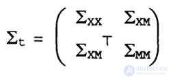
In this equation, ∑ _xx is the covariance of the data about the pose of the robot, which has already been considered in the context of localization; ∑ _xx is a 3x2n matrix that expresses the correlation between the characteristics on the map and the coordinates of the robot. Finally, ∑ _xx is a 2nx2n matrix that specifies the covariance of the characteristics on the map, including all pairwise correlations. Therefore, the need for memory for algorithms based on the EKF method is measured by the quadratic dependence on n (the number of characteristics on the map), and the update time is also determined by the quadratic dependence on n.

Before proceeding to the study of mathematical calculations, we consider the solution of the problem according to the EKF method on the graphs. The figure below shows how the robot moves in an environment with eight marks arranged in two rows of four marks each. Initially, the robot has no information about where the marks are located. Each mark is assumed to have a different color, and the robot can reliably distinguish them from each other. The robot begins to move to the left, in a predetermined direction, but gradually loses confidence in whether it has reliable information about its location. This situation is shown in Figure a) with the help of error ellipses, whose width increases as the robot moves further. The moving robot receives data on the range and azimuth to the nearest marks, and these observations are used to obtain estimates of the location of such marks. Naturally, the uncertainty in assessing the location of these marks is closely related to the uncertainty of the robot localization. Figure b), c) shows the change in the trust state of the robot as it moves further and further in its environment.

An important feature of all these estimates (which is not so easy to notice when considering the graphical images shown) is that in the algorithm under consideration a single Gaussian distribution is maintained over all estimates. The error ellipses in the figure are the projections of this Gaussian distribution onto the subspace of the robot coordinates and elevation. This multidimensional Gaussian distribution of a posteriori probabilities maintains correlations between all estimates. This remark becomes important when trying to understand what is happening in Figure d). This figure shows that the robot detects a mark previously mapped. As a result, its own uncertainty decreases sharply. The same phenomenon occurs with the uncertainty of all other marks. This event is a consequence of the fact that the assessment of the location of the robot and the assessment of the locations of the marks have a high degree of correlation in the Gaussian distribution of a posteriori probabilities. Reliable identification of knowledge about one variable (in this case, the pose of the robot) automatically leads to a decrease in the uncertainty of all other variables.

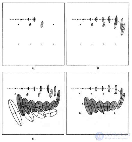
Application of the EKF method for solving the problem of mapping by a robot. The path of the robot is indicated by a dashed line, and its assessment of its own position is indicated by shaded ellipses. Eight distinguishable marks with unknown locations are shown as small dots, and estimates of their location are shown as white ellipses: the robot’s uncertainty regarding its position increases, as well as its uncertainty regarding the marks it encounters; stages during which the robot meets new marks and maps them with increasing uncertainty (a — b); the robot again meets the first mark, and the uncertainty of all marks decreases due to the fact that all these estimates are correlated (d)

The mapping EKF algorithm resembles the EKF localization algorithm described in the previous section. The main difference between them is determined by the fact that additional variable elevations are taken into account in the distribution of posterior probabilities. The motion model for grades is trivial because they do not move. Thus, for these variables, the function f is a single function, and the measurement function is essentially the same as before. The only difference is that the Jacobian H _t in the EKF update equation is taken not only in relation to the position of the robot, but also in relation to the location of the mark that was observed at time t. The resulting EKF equations are even more daunting in their complexity than those that were formulated before that; it is for this reason that we omit them here. However, there is another difficulty that has so far been ignored by us - the fact that the size of the map is M   not known in advance. Therefore, the number of elements in the final estimate µ _t and ∑ _t is also not known. This data has to be redefined dynamically, as the robot finds more and more new marks. But this problem can be solved very simply - as soon as the robot detects a new mark, it adds a new element to the distribution of a posteriori probabilities. If the value of the variance of this new element is initialized by a very large number, then the resulting distribution of a posteriori probabilities becomes the same as if the robot knew in advance about the existence of this mark.