Dynamics and control

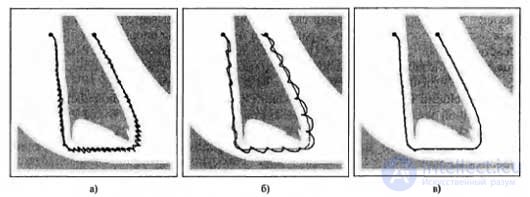
In the plans developed (especially in those that were compiled using deterministic path planners), it was assumed that the robot could simply follow any path formed by the algorithm. But in the real world, of course, things are different. Robots have inertia and cannot execute arbitrary motion commands along a given path, except at arbitrarily low speeds. In most cases, the robot, executing motion commands, makes efforts to move to a particular point, and not just sets the positions it needs. This section describes methods for calculating such efforts.

Dynamics and control

The concept of a dynamic state , which expands the concept of the kinematic state of the robot, allowing you to simulate the speed of the robot. For example, in the description of the dynamic state, in addition to data about the angle of rotation of the hinge of the robot, the rate of change of this angle is reflected. The transition model for any representation of the dynamic state takes into account the effects of effort on this rate of change. Such models are usually expressed using differential equations that associate a quantity (for example, the kinematic state) with a change in this quantity over time (for example, speed). In principle, it would be possible to choose a way to plan the movements of the robot using dynamic models instead of kinematic models. This methodology leads to the achievement of excellent performance indicators of the robot, if you can make the necessary plans. However, the dynamic state is much more complicated compared to the kinematic space, and due to the large number of measurements, the tasks of motion planning become intractable for any robots except the simplest ones. For this reason, practical robot systems are often based on the use of simpler kinematic path planners.

A generally accepted method of compensating for the kinematic plan limitations is to use a separate mechanism, a controller , for tracking the robot. Controllers are devices that generate commands to control the robot in real time using feedback from the environment to achieve the control goal. If the goal is to keep the robot on a pre-planned path, then such controllers are often called reference controllers , and the path is called a reference path . Controllers that optimize the global cost function are called optimal controllers . Essentially, the optimal policy for the MDP task is to determine the optimal controller.

At first glance, the control task, which allows the robot to keep on a predetermined path, seems relatively simple. But in practice, even while solving this seemingly simple task, some pitfalls can occur. Figure a) shows which violations may occur. This figure shows the path of the robot attempting to follow the kinematic path. After the occurrence of any deviation (due either to noise or restrictions on the efforts that the robot can apply), the robot applies an opposing force, the magnitude of which is proportional to this deviation. Intuitive ideas suggest that this approach is supposedly fully justified, since the deviations must be compensated by the opposing effort so that the robot does not deviate from its trajectory. However, as shown in a) , the actions of such a controller cause a rather intense vibration of the robot. This vibration is the result of the natural inertia of the robot arm - the robot, sharply directed to the sides of the reference position, slips through this position, which leads to the appearance of a symmetrical error with the opposite sign. According to the curve shown in figure a) such overshoot can continue along the entire trajectory, therefore the resultant movement of the robot is far from ideal. Obviously, you need to provide a better way to manage.

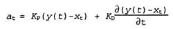
Control the robot arm using various methods: proportional control with a gain of 1.0 (a); proportional control with a gain of 0.1 (b); proportional differential control with gains of 0.3 for the proportional and 0.8 for the differential component (c). In all cases, an attempt is made to navigate the robot arm along the path marked in gray.

In order to understand what the best controller should be, let us formally describe the type of controller that allows overshoot. Controllers that apply inversely proportional to the observed error are called P-controllers . The letter P is short for proportional (proportional) and indicates that the actual control action is proportional to the positioning error of the robot arm. As a more formal statement, let us assume that y (t) is a reference path, parameterized by the time index t . The control action a _t produced by the P-controller has the following form:

a _t = K _p (y (t) -x _t )

where x _t is the state of the robot at time t; K _P - the so-called coefficient

the gains of the controller, on which depends, what effort the controller will apply, compensating for deviations between the actual state x _t and the desired y (t). In this example, CR = 1. At first glance it may seem that the problem can be fixed by choosing a smaller value for the RC. But, unfortunately, the situation is different. Figure b) shows the trajectory of the robot arm at K _P = .1, in which the oscillatory behavior still manifests itself. Reducing the magnitude of the gain contributes only to a decrease in the intensity of oscillations, but does not eliminate the problem. In fact, in the absence of friction, the P-controller acts in accordance with the law of the spring, so it oscillates to infinity around a given target point.

In traditional science, tasks of this type belong to the field of control theory, which is becoming increasingly important for researchers in the field of artificial intelligence. Research in this area, conducted over decades, has led to the creation of many types of controllers, far superior to the controller described above, which operates on the basis of a simple control law. In particular, the reference controller is called stable if small disturbances result in a limited error connecting the robot signal and the reference signal. A controller is said to be strictly stable if it is able to return the device it controls to the reference path after exposure to such disturbances. It is obvious that the P-controller considered here only appears to be outwardly stable, but is not strictly stable, since it is not capable of ensuring the return of the robot to its reference trajectory.

The simplest controller, which allows to achieve strict stability in the conditions of this task, is known as the PD controller . The letter P is again an abbreviation of proportional (proportional), a D - of the derivative (differential). To describe PD controllers, the following equation applies:

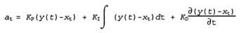
According to this equation, PD controllers are P-controllers, supplemented by a differential component, which adds to the control value at a term proportional to the first derivative of the error y (t) -xt over time. What is the result of adding such a term? Generally speaking, the differential term quenches the oscillations in the system to control which it is used. To verify this, consider the situation in which the error (y (t) -xt) changes dramatically over time, as was the case with the P-controller described above. In this case, the derivative of such an error is applied in the direction opposite to the proportional term, which leads to a decrease in the overall response to the perturbation. However, if the same error continues its presence and does not change, then the derivative will decrease to zero and the proportional term will dominate the selection of the control action.

The results of applying such a PD-controller to control the robot arm when used as gain factors values ​​K _P =. 3 and K _D =. 8 are shown in figure c) . Obviously, in the end, the trajectory of the manipulator has become much smoother and there are no visible fluctuations on it externally. As this example shows, the differential term allows you to ensure the stability of the controller in those conditions when it is unattainable in other ways.

But, as practice shows, PD-controllers also create prerequisites for failures. In particular, PD controllers may not be able to adjust the error to zero, even in the absence of external disturbances. This conclusion does not follow from the example of the robot in this section, but, as it turned out, sometimes it is necessary to apply feedback with proportional overshoot to reduce the error to zero. The solution to this problem is that you need to add a third term to the control law, based on the results of the integration of the time error:

where K _t is another gain. In the term ∫ (y (t) -x _t ) dt , the integral of the error over time is calculated. Under the influence of this term, the long-term deviations between the reference signal and the actual state are corrected. If, for example, x _{t is} less than y (t) for an extended period of time, then the value of this integral increases until the resulting control action a _t causes a decrease in this error. Thus, the integral terms guarantee the absence of systematic errors in the actions of the controller by increasing the risk of oscillatory behavior. The controller, the control law of which consists of all three terms, is called the P ID controller . PID controllers are widely used in industry for solving various control tasks.