Localization

Localization is a universal example of robotic perception. It is the task of determining where things are. Localization is one of the most common tasks of perception in robotics, since knowledge about the location of objects and the actor himself is the basis of any successful physical interaction. For example, robots of the type of manipulators must have information on the location of the objects they manipulate. And robots moving in space must determine where they themselves are in order to pave the way to the target locations.

There are three types of localization problem with increasing complexity. If the initial pose of the object being localized is known, then localization is reduced to the task of tracing the trajectory . Trajectory tracking tasks are characterized by limited uncertainty. More difficult is the task of global localization , in which the initial location of the object is completely unknown. The tasks of global localization are transformed into tasks of tracing the trajectory immediately after the localization of the desired object, but in the process of solving them there are also such stages when the robot has to take into account a very wide list of undefined states. Finally, circumstances can play a cruel joke with the robot and an “abduction” (i.e., a sudden disappearance) of the object, which he tried to locate, will occur. The task of localization in such uncertain circumstances is called the task of abduction . A kidnapping situation is often used to test the reliability of a localization method in extremely adverse conditions.

In order to simplify, suppose that the robot is slowly moving on a plane and that it is given an exact map of the medium. The position of such a mobile robot is determined by two Cartesian coordinates with x and y values, as well as its angular direction with a value of 0, as shown in Figure a) . (Note that the corresponding speeds are excluded.

therefore, the model under consideration is rather kinematic rather than dynamic.) If these three values ​​are ordered in the form of a vector, then any particular state will be determined using the relation xt = (x _t , y _t , 0 _t ) ^t .

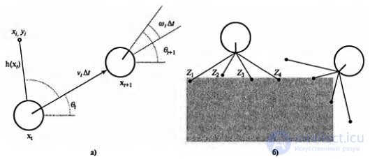
Application example of the environment map: a simplified kinematic model of a mobile robot. The robot is shown as a circle with a mark indicating the forward direction. The values ​​of position and orientation at times t and t + 1 are shown, and updates are indicated by the terms v _t Δ _t and w _t Δ _t, respectively. In addition, the mark with the coordinate (x _i , y _i ), observed at the time t (a); distance sensor model. Two poses of the robot are shown corresponding to the specified distance measurement results (z _1, z ₂ , z ₃ , z ₄ ). Much more likely is the assumption that these distance measurement results are obtained in the pose shown on the left rather than on the right (b)

In this kinematic approximation, each action consists of an “instantaneous” specification of two speeds — the transfer velocity v _t and the rotation speed w _t . For small time intervals ∆ _{t, the} coarse deterministic motion model of such robots is given as follows:

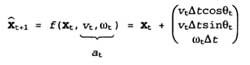
The designation x refers to deterministic state prediction. Of course, the behavior of physical robots is rather unpredictable. This situation is usually modeled by a Gaussian distribution with mean f (x _t , v _t , w _t ) and covariance ∑ _x. .

P (x _{t +1} | x _t , w _t ) = N (x _{t +1} , _x )

Then you need to develop a model of perception. Consider the model of perception of two types. In the first of these, it is assumed that the sensors detect stable, distinguishable environmental characteristics, called elevations . For each mark, they report range and azimuth. Suppose that the state of the robot is determined by the expression x _t = (x _t , y _t , 0 _t ) ^T and it receives information about the elevation whose location, as is known, is determined by the coordinates (x _i , y _i ) ^T. In the absence of noise, the range and azimuth can be calculated using a simple geometric ratio. An accurate prediction of the observed range and azimuth values ​​can be made using the following formula:

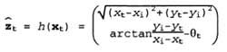
Once again, we note that the results of measurements are distorted by noise. For simplicity, we can assume the presence of Gaussian noise with the covariance ∑ _z :

P (z _t   | x _t ) = N (z _t , ∑ _z )

For range finders, a slightly different perception model is often more acceptable. Such sensors produce a vector of values ​​of the range z _t   = (z ₁ , ...., z _M ) ^t , in each of which the azimuths are fixed with respect to the robot. Provided that the pose x _{t is given} , suppose that

z _j   - the exact distance along the direction of the j-ro beam from x _t to the nearest obstacle. As in the previously described case, these results may be distorted by Gaussian noise. As a rule, it is assumed that the errors for different directions of the rays are independent and are given in the form of identical distributions, therefore the following formula holds:

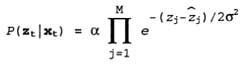
Figure b) shows an example of a four-beam range finder and two possible robots, one of which can be completely considered as a pose in which the considered measurement results were obtained, and the other is not. Comparing the model of measuring distances with the model of marks, one can be convinced that the model of measuring distances has the advantage that it does not require the identification of a mark in order to be able to interpret the results of measuring distances; and indeed, as shown in figure b) , the robot is directed toward the wall, which has no characteristic features. On the other hand, if there was a visible, clearly identifiable mark in front of it, the robot could provide immediate localization. A Kalman filter is described that allows you to represent a trusting state in the form of a single multi-dimensional Gaussian distribution, and a particle filter that represents a trusting state in the form of a collection of particles corresponding to the state. Most modern localization algorithms use one of these two representations of the trust state of the robot, P (x _t | z _{1: t} , a _{1: t-1} ).

Localization using particle filtering is called Monte Carlo localization , or MCL (Monte Carlo Localization). The MCL algorithm is identical to the particle filtering algorithm shown in the listing; it is enough to provide a suitable movement model and perception model. One of the versions of the algorithm in which the model of measuring distances is used is shown in the listing. The operation of this algorithm is shown in the figure below, where it is shown how the robot determines its location in an office building. In the first image, the particles are evenly distributed according to the distribution of a priori probabilities, indicating the presence of global uncertainty regarding the position of the robot. The second image shows how the first row of measurement results arrives and the particles form clusters in areas with a high distribution of a posteriori confidence states. And in the third image it is shown that a sufficient number of measurement results arrived in order to move all particles to one place.

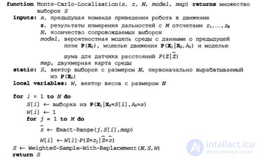
Listing . Monte-Carlo localization algorithm, which uses the model of perception of the results of measuring distances, taking into account the presence of independent noise

Another important method of localization is based on the use of a Kalman filter. The Kalman filter represents the posterior probability P (x _t | z _{1: t} , a _{1: t-1} ) using the Gaussian distribution. The average of this Gaussian distribution will be denoted by μ _t , and its covariance - ∑ _t . The main disadvantage of using Gaussian confidence states is that they are closed only when using linear models of motion f and linear models of measuring h. In the case of nonlinear f or h, the result of updating the filter is usually not Gaussian. Thus, localization algorithms in which the Kalman filter is used linearize the models of movement and perception. Linearization is a local approximation of a nonlinear function using a linear one.

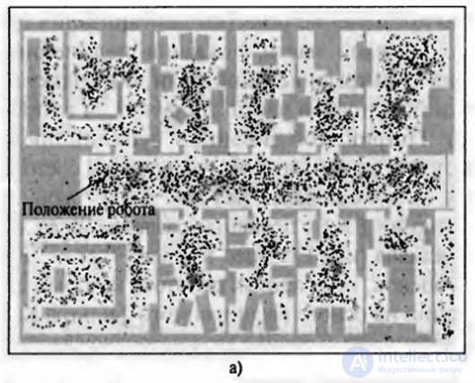
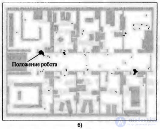
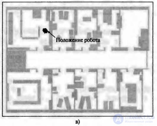
Monte-Carlo localization method based on particle filtering algorithm for localizing a mobile robot: initial state, global uncertainty (a); approximately bimodal state of uncertainty after passing through the (symmetric) corridor (b); Unimodal state of uncertainty after the transition to the office, distinguishable from others (c)

Figure 1 shows the application of the concept of linearization for a (one-dimensional) model of the robot's motion. The left side shows the nonlinear model of motion f (x _t , a _t ) (the a parameter _t on this graph is not shown, since it does not play any role in this linearization). On the right side, this function is approximated by a linear function f (x _t , a _t ). The graph of this linear function is tangential to the curve f at the point μ _t , which determines the average estimate of the state at time t. This linearization is called Taylor expansion (first degree). The Kalman filter, which linearizes the functions f and h using a Taylor expansion, is called an extended Kalman filter (or Extended Kalman Filter — EKF). Figure 2 shows the sequence of estimates obtained by the robot, which operates under the control of a localization algorithm based on an extended Kalman filter. As the robot moves, the uncertainty in estimating its location increases, as shown by error ellipses. But as soon as the robot begins to receive data on the range and azimuth to the mark with a known location, its error decreases. Finally, the error increases again as soon as the robot loses sight of it. The EKF algorithms are successful if the tags are easily identifiable. Another option is that the posterior probability distribution can be multimodal. A task for which you want to know the identification of marks is an example of a data association task.

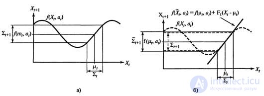
Figure 1. One-dimensional illustration of the linearized motion model: the function f, the projection of the mean μ _t and the covariance interval (based on ∑ _t ) at the time t + 1 (a); The linearized version is tangent to the curve of the function f with the value of μ _t . The projection of the mean µ _{t is} defined correctly. However, the covariance projection ∑ _{t + 1} differs from ∑ _{t + 1} (b)

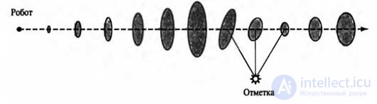
Figure 2. Example of localization using the advanced Kalman filter. The robot moves in a straight line. As it progresses, the uncertainty gradually increases, as shown by error ellipses. And after the robot detects a mark with a known position, the uncertainty decreases.