Antenna Radiation Resistance

Radiation resistance — is a quantity that has the dimension of resistance and relates the radiated power P_rad to the current I_A flowing through some cross-section of the antenna. Radiation resistance is used to determine the power consumption of the antenna.

Radiation resistance is usually determined in terms of the current at the antinode

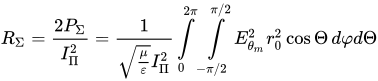(1)

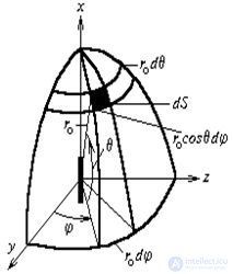
Here P_Σ — the time-averaged radiated power; I_Π — the amplitude of the current at the antinode; r,Θ,φ — the coordinates of the spherical system (Fig.1). Substituting into (1), in place of E_Θm = E_m, from the expression

we can write:

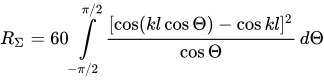(2)

Integrating (2) leads to the following formula for the radiation resistance of a dipole:

(3)

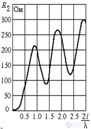
Fig.2 — Radiation resistance

where C = 0.577 is Euler's constant; 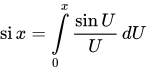— the sine integral; 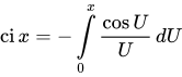— the cosine integral. It follows from formula (3) that the radiation resistance of a symmetrical dipole depends only on the ratio . In practice, however, the radiation resistance also depends on the location of the antenna relative to the Earth and surrounding objects.

The results of computing R_Σ by formula (3), as a function of , are shown on the graph (Fig.2).

Each element of a transmitting antenna participates in radiation, emitting a partial power Δp (Fig. 2.55). The sum of all the powers of all the partial elements constitutes the resulting energy flow. The partial radiated power of an element Δl depends on the location of the element on the antenna, since the values of the currents passing through the various elements differ and, in addition, depend on the value of the current IA supplied to the input terminals (clamps) of the antenna.

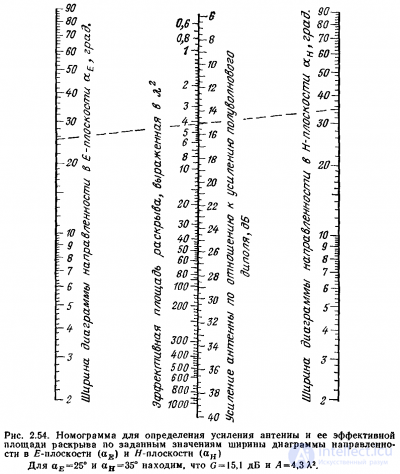
Fig. 2.54. Nomogram for determining antenna gain and its effective aperture area from given values of the beamwidth of the radiation pattern.

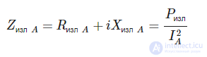
Taking the ratio of the power Prad to the square of the current, we obtain that at points A — A

(2.132)

In resonant antennas, the radiation resistance, called the characteristic resistance, is referred to the points corresponding to the maximum value of the current.

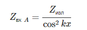
For an infinitely thin antenna, on which the current distribution is sinusoidal, both resistances are related to each other by the dependence

(2.133)

where ZinA — the input impedance of the antenna relative to points A—A, Zrad — the radiation resistance of the antenna; kx — the phase distribution from the feed point to the point corresponding to the maximum value of the current.

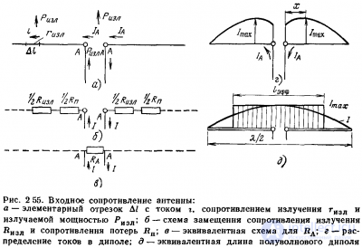
Fig. 2.55. Input impedance of the antenna.

(2.134)

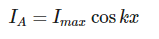
The current passing through the input terminals of the antenna, where Imax — the maximum value of the current.

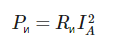
The current flowing through an antenna made of a material with finite conductivity σ dissipates thermal power

(2.135)

where IA — the current in the antenna; Rloss — the loss resistance in the antenna. The loss resistance Rloss depends not only on the conductivity σ of the material, but also on the nature of the current distribution over the antenna.

The sum of both resistances (the loss resistance and the radiation resistance) constitutes the input impedance of the antenna.

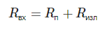(2.136)

The concept of input impedance can also be applied to a receiving antenna. For a receiving antenna, the relation holds

(2.137)

where η — the efficiency. It follows from this formula that an antenna having a larger value of radiation resistance Rrad also has a larger value of efficiency.

Note that, for the power source, the antenna represents a resistance

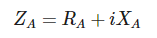(2.138)

For an antenna tuned to resonance, the impedance ZA has only a real component (XA = 0). With a slight detuning of the antenna from resonance (for example, by changing the frequency or the length of the antenna), a substantial increase in XA is observed at a practically constant value of RA.

Let us give typical values of the input impedance of antennas having length l and made of wire of diameter d:

• half-wave dipole.....RA=60÷75 Ohm
• full-wave dipole.......RA=600÷3000 Ohm
• folded dipole.......RA=230÷300 Ohm

The data given are valid provided that 70≤l/d≤10 000.

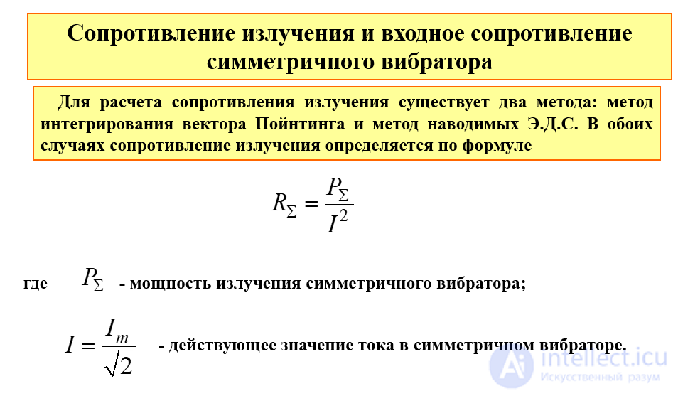
fig. Radiation resistance and input impedance of a symmetrical dipole

Radiation resistance and effective height of an antenna

The resistive component at the feed points is called the radiation resistance R_Σ, since in a transmitting antenna it corresponds precisely to the useful loss of the supplied power to radiation. In the case of a receiving antenna, it is the internal resistance of that equivalent generator which develops the EMF we calculated, ε = E • h_eff. It now becomes clearer with what the input impedance of the detector must be matched.

The effective height of an antenna is obtained from the following considerations (Fig. 2.14): if the current did not vary along the height of the antenna, then to obtain the same radiation (and reception) efficiency the antenna would have to have a height h_eff. Mathematically, the effective height is obtained by integrating the current distribution function. For a quarter-wave vertical antenna, h_eff = λ / 2π = 0.641L_A. For short vertical antennas, the current distribution approaches triangular, and the effective height approaches half the geometric height, h = 0.5 L_A.

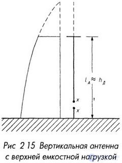
Attempts to increase the natural wavelength of an antenna without increasing its height led to the appearance of antennas with top capacitive loading. An L-shaped (inverted-L) antenna is obtained from a vertical one if its upper part is bent at a right angle and directed horizontally. The current distribution on the wire remains the same, but only the vertical part will receive waves with vertical polarization. The effective height thereby approaches the geometric height of the antenna's suspension the more, the more developed the horizontal part is. The current distribution in a vertical antenna with a horizontal part or any other top capacitive loading is shown in Fig. 2.15. For such antennas λ₀ = k • L_A, where L_A should be understood as the total length of the vertical part and all conductors of the horizontal part, and the coefficient k is determined approximately from Table 2.1.

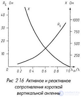
In most cases, the wavelength at which the antenna operates is significantly greater than its natural one, and the impedance is complex in nature, with resistive and reactive components determined by the formulas: Z_A = R_Σ - jX, R_Σ = 1600 (h_eff/λ)², X = W ctg (πλ₀/2λ), where W is the characteristic impedance of the antenna wire, equal to approximately 400-600 Ohm (increasing for thin wires). Approximate dependences of these impedances for a thin vertical antenna with top capacitive loading on the ratio λ₀/λ are shown in Fig. 2.16.

Table 2.1 Coefficients for determining the natural wavelength of an antenna

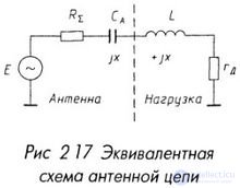
fig Equivalent circuit of the antenna circuit

For antennas operating on waves longer than their natural one, the reactance is capacitive in nature, increasing sharply as the antenna is shortened (since the capacitance decreases). To compensate for it, an inductance (a loading coil) is included in the antenna circuit, and the equivalent circuit of the antenna circuit takes the form shown in Fig. 2.17. Note that it is in no way different from the circuit of an oscillatory (resonant) circuit tuned to resonance with the frequency of the EMF source! The Q-factor of the resulting circuit can be very high, since the reactance is much greater than the resistance.

See also

• [[b348]]

See also

• 5 Structural diagram of the antenna. Antenna classification. Characteristics of antennas in the transmitting and receiving modes. The reciprocity theorem and its application in the theory of receiving antennas