Models of short-term aggregate labor supply

Model hard nominal wage

The fundamentals of a rigid nominal wage model were laid by J.M. Keynes. It was further developed in the works of the well-known contemporary American economist, former Managing Director of the International Monetary Fund, one of the authors of the most popular textbooks on economic theory and especially on macroeconomics Stanley Fisher. (It should not be confused with the already well-known American economist of the first half of the twentieth century, Irving Fisher - the author of the "Fisher equation", the "Fisher effect" and the "Fisher index").

The rigidity of the nominal wage rate is explained by the institutional features of the modern economy and the functioning of the labor market, namely:

• employment contracts (for the duration of the contract, that is, for 1-3 years, the nominal wage rate cannot be revised);
• the activity of trade unions and collective agreements (in contracts between trade unions and entrepreneurs, a nominal wage rate is fixed, below which firms do not have the right to hire workers);
• state laws on the minimum wage (the firm has no right to hire a worker at a rate below the minimum state established by the state)
• the theory of effective wages (it is unprofitable for firms to pay low wages, and even less to reduce the nominal rate, since wages are viewed as a tool for motivating labor and increasing its productivity).

We derive the short-term aggregate supply curve graphically (Fig. 1).

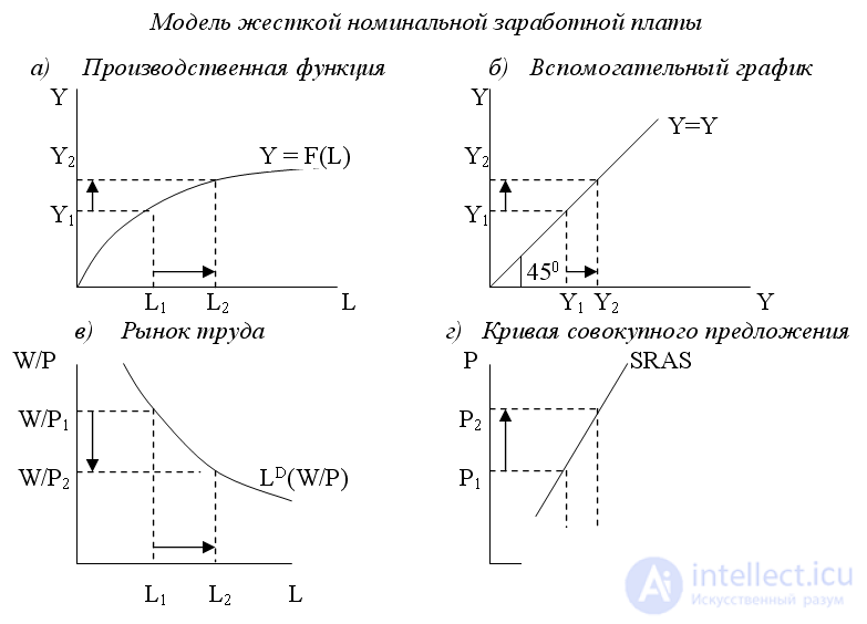
Suppose that the economy is initially in a state of full employment, i.e. L ₁ = L _F and Y ₁ = Y *. With an increase in the price level (from P ₁ to P ₂ ) under the conditions of a constant nominal wage rate (W), the real wage rate (W / P), which determines the value of firms' demand for labor, decreases (W / P ₂ <W / P ₁ ), which makes labor cheaper.

The lower real wage rate contributes to the fact that firms hire more workers (in the labor market (Fig. 16.6. (C)) the magnitude of the demand for labor increases from L ₁ to L ₂ ). A greater amount of labor used in production, in accordance with the production function (Fig. 16.6. (A)) leads to an increase in the output of products by firms and an increase in the total volume of production (from Y ₁ to Y ₂ ). Thus, the increase in the price level (from P ₁ to P ₂ ) led to an increase in output (from Y ₁ to Y ₂ ), i.e. there is a direct relationship between the price level and the volume of output, therefore, the aggregate supply curve in the short-term period, while the nominal wage is unchanged, has a positive slope (Fig. 1 (d)). Since the change in the price level occurred both for workers and for firms unexpectedly, the equation of this curve: Y = Y * + α (Р - Р ^e )

The actual release exceeded the potential due to the unexpected increase in the price level.

Model of employee misconceptions

A model of employee misconceptions as an explanation of the positive inclination of the short-term aggregate supply curve was proposed in the 60s by the head of the monetarist trend in economic theory, the founder of the theory of adaptive expectations by the famous American economist M. Friedman and his colleague Edmund Phelps. The main idea of ​​this model is that workers temporarily confuse the concept of nominal and real wages and perceive the increase in the nominal wage rate associated with an increase in the price level as an increase in their real wages. Therefore, labor supply increases, which leads to an increase in output in the short term until workers understand the fallacy of their assumptions and make sure that their real wages decrease, as the rise in price levels outpaces the growth of nominal wages. In this case, only workers are mistaken (it is not by chance that this model is called the “fooling model” - the “fooling” (workers) model). Firms always correctly represent the ratio of growth rates of prices and nominal wages and in the case when prices rise faster than nominal wages, which means a decrease in real wages, increase the demand for labor, which leads to an increase in output. Graphically, the model of employee misconceptions is shown in Fig. 2

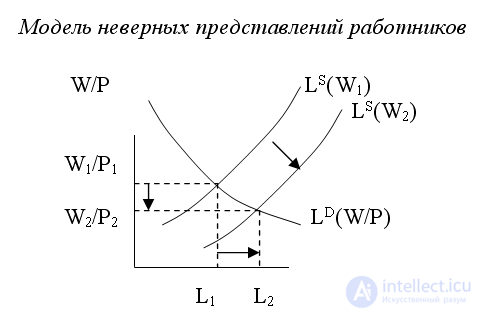
Consider the behavior of workers. As the nominal wage increases from W ₁ to W ₂ , the labor supply increases (the labor supply curve L ^S (W ₁ ) shifts to the right to L ^S (W ₂ )), as a result employment increases from L ₁ to L ₂ , which leads to growth in total output (see Figure 2), and the real wage rate is falling (from W 1/1 to W ₂ / P ₂ ).

It should be borne in mind that, in principle, workers (in accordance with the prerequisites of the monetarist model) have no monetary illusions, i.e. in offering their labor, they are guided by the real (and not nominal) wage rate. However, workers' mistakes are based on the fact that they do not know the relationship between the growth rates of nominal wages and the price level and, when signing a contract, they are guided by the price level that exists at that moment in the economy (P ₁ ) without waiting for its change. Therefore, in the opinion of the workers, the growth of nominal wages corresponds to the growth of their real wages, and therefore they increase the supply of labor.

If the price level unexpectedly for workers rises to P ₂ , then this means that the actual price level was higher than expected, and if the price level increase (ΔP) exceeds the growth of nominal wages (ΔW), then the real wage is reduced (W ₂ / P ₂ <W ₁ / P ₁ ), but the workers discover this with some lag (delay).

Because firms are well aware of the relationship between price and nominal wage growth rates, and know that real wages have fallen, they hire more workers (the demand for labor increases, which in the graph corresponds to the movement along the demand curve for labor) and increase output . As a result of an increase in the supply of labor and the growth in the magnitude of the demand for labor, the volume of production is growing in the short run. If we assume that the economy is initially in a state of full employment, then the deviation of the actual output from the potential will occur due to the discrepancy between the actual price level and the expected by workers, i.e. can be calculated by the formula: Y = Y * + α (Р - Р ^e )

Imperfect Information Model

This model belongs to the well-known American economist, Nobel laureate Robert Lucas, who explained the possibility of deviation of output in the short term from its potential level by the fact that firms are mistaken. The imperfect information model comes from the premise that each producer in the economy produces only one product, and there are many consumers. According to Lucas, the economy is similar to an archipelago consisting of individual islands (manufacturing companies) that practically do not communicate with each other and do not have information about what is happening on other islands and in the archipelago as a whole, but which are periodically visited by consumers buying goods . Therefore, manufacturers are able to track price changes only for their product, and not for all others.

Therefore, when the prices of goods rise, manufacturers (firms) perceive price increases for their own goods not as a manifestation of an increase in the general price level, but as an increase in the price only of their goods relative to prices for other goods, i.e. as a relative price increase. And since the price of goods produced by a firm has increased, it increases production, believing that the relative price of its goods has increased. This leads to an increase in total output.

Thus, due to the incompleteness and imperfection of information, firms confuse changes in the general price level with changes in relative prices, and as a result, in the short term, until firms find their mistake and do not face the fact that they have to buy all the goods necessary for production at increased prices, they will increase output. So, the increase in the price level leads to an increase in production. Since the increase in prices for goods, including for the goods produced by the company, occurs unexpectedly for it (the actual price becomes higher than the expected one), this causes a temporary (in the short term) excess of the actual output over its potential level, which may be expressed by the formula: Y = Y * + α (Р - Р ^e )

Hard Price Model

This model was proposed and substantiated by representatives of the neo-Keynesian trend in economic theory. The model of rigid (inflexible) prices is based on the assumption that firms do not immediately change the prices of their products in response to fluctuations in demand. This is due to the following reasons:

• prices may be negotiated between firms and customers;
• firms are afraid to scare away the frequent price changes of their regular customers
• A firm may fear high “menu costs” caused by price changes and associated with the need to reprint (reprint) and send out catalogs and price lists, as well as advertising new prices.

Therefore, with the growth of aggregate demand, firms increase production, and some firms do not raise prices for their products for some time. However, the remaining part of firms (and, as a rule, most of them) in the conditions of increased demand for their products, on the one hand, increases output, and, on the other hand, increases prices for it. As a result, the general price level begins to rise. This leads to an increase in the costs of firms, which requires them to establish a higher price for their products. As a result, the actual price level is higher than expected by firms that maintain tight prices, and the volume of production is greater than the potential level of output. We again obtain the formula for the value of output (aggregate supply) in the short term:

Y = Y * + α (Р - Р ^e )

So, all four models give a general conclusion and a general final formula for the value of aggregate supply in the short run. It follows from the equation that the short-term aggregate supply curve has a positive slope, and the deviations of the actual output from the potential are due to deviations of the actual price level from the expected one.

Transition from short-term to long-run equilibrium

Consider what happens if aggregate demand unexpectedly increases in the economy (Fig. 3). In accordance with the AD-AS model, in the short run, the equilibrium of the economy will move from point A to point B. The growth of aggregate demand (shift of the aggregate demand curve from AD ₁ to AD ₂ ) will lead to an increase in the price level higher than expected (P ₂ > P ₁ ) and respectively, to the growth of output above potential level (Y ₁ > Y *).

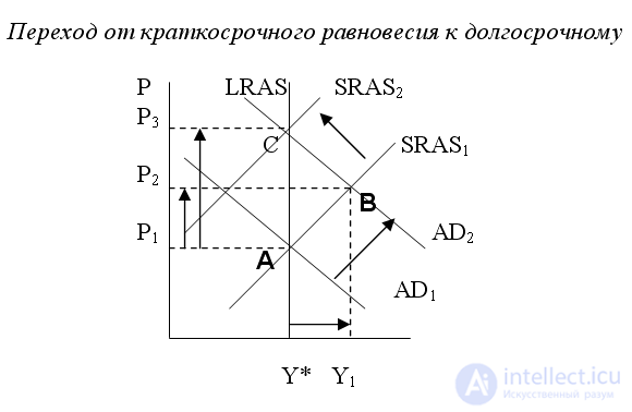
In the long run, the expected price level rises (workers and firms adjust their expectations) and the short-term aggregate supply curve shifts upwards (from SRAS ₁ to SRAS ₂ ). Equilibrium moves from point B (point of short-term equilibrium) to point C (point of long-term equilibrium). The economy returns to potential output, but at a higher price level (P ₃ > P ₁ ).

Thus, the transition from a situation of short-run equilibrium to a state of long-run equilibrium is due to the adjustment of expectations. When the actual price level coincides with the expected price level, the actual output is equal to the potential one, and the economy is on a long-term aggregate supply curve. This corresponds to the Lucas equation: Y = Y * + α (P - P ^e ), i.e. if P = P ^e , then Y = Y *.