Lecture
The basis for constructing the IS curve is: 1) the model of total expenditures (the Keynesian cross model), discussed in Chapter 12, which shows what determines the income in the economy at a given level of planned expenditures (that is, it comes from the premise that the level of autonomous costs are fixed); 2) the function of dependence of autonomous planned expenses on the interest rate.
Since the model includes a new endogenous variable — the interest rate — we will consider it in more detail. Interest rate and autonomous costs. For savers, the interest rate acts as a reward for abstaining from current consumption against expected future consumption. For borrowers, the interest rate is the price of borrowed money used by investors to buy investment goods, and households to buy consumer durables. In economics, there are many specific types of interest rates, such as interest rates paid:
In economic theory, identifying the main, fundamental relationships and interdependencies in the economy, the differences between different types of interest rates are assumed to be insignificant, and the market interest rate is the average of all the different rates.
The ratio between autonomous planned expenditures and interest rates. The change in interest rate affects the following components of autonomous costs:
• investment costs. Borrowing funds for the purchase of investment goods, firms are trying to make a profit. Therefore, they invest in equipment and industrial facilities (acquire real capital) as long as the rate of return on an additional unit of capital exceeds the cost of borrowed funds for the purchase of this additional unit, i.e. interest rate. Any increase in interest rates reduces the effectiveness of investment projects. Therefore, if the interest rate is so high (the credit funds of the road) that the expected rate of return is lower than this rate, the firm will refuse to implement such an investment project and the amount of investment expenses will decrease. Consequently, the relationship between the value of investment spending and the interest rate is the opposite. The higher the interest rate, the less the firms desire to invest. The investment function can be written: I = I ( R ) or, if the dependence is linear:
I = I - dR, where I - autonomous investments, R - interest rate, d - coefficient reflecting the sensitivity of investment expenditures to the interest rate and showing how much the investment expenditures change when the interest rate changes by one percentage point. The coefficient is d> 0, and since there is a minus sign in the formula, the curve has a negative slope.
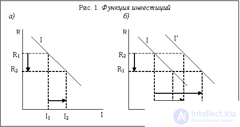
The curve of aggregate investment demand (Fig. 1. (a)) reflects this inverse relationship between the magnitude of the demand for investment and the interest rate.
The shift in the curve of total investment costs occurs when the value of autonomous investments (I) changes: their increase shifts the curve to the right, and their reduction shifts to the left. These changes, as a rule, are attributed by representatives of the Keynesian sector to the mood of investors, a pessimistic or optimistic assessment of the expected profitability of investment expenses. The consequences of an increase in the level of autonomous investments are shown in Fig. 1. (b) shift of the curve I to the right to I '.
The slope of the curve of total investment costs due to the value of the coefficient d; than he is taller, i.e. the more sensitive investments are to changes in interest rates, the more gentle curve I is: even minor changes in interest rates lead to significant changes in the value of investment demand.
• consumer spending. Similarly to investors, households also use borrowed funds, especially when purchasing consumer durable goods. Consumers compare interest payments on debt (consumer credit) with the desire to purchase a product (for example, a car or a dishwasher) as soon as possible. High interest rates are forcing some consumers to postpone the purchase until better times and autonomous consumer spending is declining. Thus, the relationship between total autonomous consumer spending and the interest rate is inverse and all the reasoning and conclusions are similar to those made regarding investment costs (not by chance, some economists suggest considering expenditures on consumer durable goods as household investment expenses). Thus, consumer spending depends not only on the level of disposable income, but also on the interest rate, and the consumer function can be represented by the formula: C = C (Y, T , t, R ) or with a linear relationship: C = C + mpc ( Y is T-tY) is aR, where C is autonomous consumer spending, Y is income, T is autonomous net taxes (taxes Tx minus transfers Tr), mpc is the marginal propensity to consume (0 <mpc <1), indicating how much consumer spending changes with a change in disposable income per unit (mpс = ΔC / ΔYd); t - the marginal tax rate (t = ΔT / ΔY), which shows the change in the value of tax revenues when the value of total income changes by one; a - the sensitivity of autonomous consumer spending to the interest rate (a> 0), reflecting the change in consumer spending when the interest rate changes by one percentage point (a = ΔC / ΔR),
• net export costs. The change in the interest rate also affects the value of net exports. The growth of the interest rate in the country increases the return on invested capital and determines the inflow of capital from abroad. As a result, the demand for the national currency of a given country in foreign exchange markets is growing, and the national currency is becoming more expensive. This leads to the fact that the goods of this country become relatively more expensive, and imported goods are relatively cheaper. The demand for national goods from foreigners is falling, reducing exports, and the demand for foreign goods is growing, increasing imports. Net exports are shrinking, reducing total costs. Consequently, there is an inverse relationship between net exports and interest rates.
Therefore, the export formula can be represented as: Xn = Xn ( Y , e ) or with a linear relationship: Xn = Ex - ( Im + mpm Y) - eR = Xn - mpm Y - eR,
where Ex is autonomous export; Im autonomous import; Хn - autonomous net export; mpm is the marginal propensity to import (0 <mpm <1), which shows how the value of expenses on the purchase of imported goods changes when income changes by one (mpm = ΔIm / ΔY); e is the sensitivity of net exports to the interest rate (e> 0), showing the change in the value of net exports, if the interest rate changes by one percentage point (ΔXn / ΔR).
IS curve construction. Since the value of planned autonomous expenses depends on the interest rate, and the overall level of real output and real income depends on the size of autonomous planned expenses, if we combine these dependencies together, we can conclude that real income should depend on the interest rate. By plotting this relationship graphically, we get the IS curve. Let's display the graph of the IS curve in two ways:
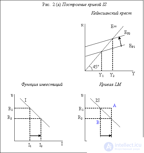
In fig. 2. (a) The IS curve is derived from the Keynesian cross and investment function. At the interest rate R 1, the value of investment expenses is equal to I 1 , which corresponds to the value of the planned expenses Ep 1 , at which the value of total income (output) is equal to Y 1 . When the interest rate decreases to R 2 , the value of investment expenses rises to I 2 , therefore, on the Keynesian cross graph, the planned expenditure curve shifts up to Ep 2 , which corresponds to the value of total income (output) Y 2 . Thus, a higher interest rate R 1 corresponds to a lower level of aggregate output Y 1 , and a lower interest rate R 2 corresponds to a higher level output Y 2 . Moreover, in both cases the product market is in equilibrium, i.e. expenses are equal to income (Ep 1 = Y 1 and Ep 2 = Y 2 ). This is reflected in the IS curve, each point of which shows paired combinations of the interest rate and income level at which the product market is in equilibrium.
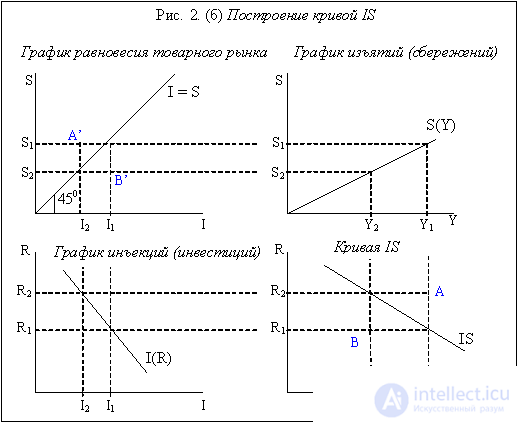
In fig. 2. (b) the IS curve is derived from the principle of equality of injections (investments) and withdrawals (savings) (which is a condition for the equilibrium of the commodity market), which follows from the basic macroeconomic identity:
C + I + G + Ex = C + S + T + Im
Subtract from both parts of the equality of consumer spending C, we get:
I + G + Ex = S + T + Im
On the right side of equality - injections - expenses that increase the flow of income, and on the left side - leakages - variables that reduce income. In an equilibrium economy, expenses are equal to income, and injections are equal to withdrawals. Injections are negatively dependent on the interest rate, and withdrawals positively depend on the level of income. Given these dependencies, you can write:
I (R) + G + Ex (R) = S (Y) + T (Y) + Im (Y)
In fig. 2. (b) 4 graphics are shown. The I graph shows the equilibrium condition of the commodity market - equality of injections (represented by investments) and withdrawals (represented by savings), which graphically reflects the bisector of the angle (line at 45 o ). Graph II presents a graph of direct dependence of withdrawals on income. The third graph shows the inverse dependence of injections on the interest rate. As a result, on the IV graph, we obtain the IS curve. At the interest rate R 1, the injection amount is I 1 , which corresponds to the size of the seizures S 1 , and this value will be at the income level Y 1 . Similarly, with the interest rate R 2, the injection amount will be equal to I 2 , at which the seizure amount will be S 2 , which corresponds to the income level Y 2 . Combining the points obtained on the IV plot with a straight line, we obtain the curve IS.
The IS curve shows all possible combinations of interest rate (R) and real income (Y) levels at which the product market is in equilibrium, i.e. the demand for goods and services is equal to their supply, which happens only when income is equal to the planned expenditures, and injections are equal to withdrawals.
Points outside the IS curve. At any point outside the IS curve, the economy is in disequilibrium. For example, in t.A (Fig. 2. (b)), which is above the IS curve, the amount of income is equal to Y 2 , which corresponds to the value of withdrawals S 2 , and the interest rate is R 1 , at which the injection value is equal to I 1 . In this case, withdrawals exceed injections (S 2 > I1), which means that in the commodity market the income (output) exceeds expenses, i.e. the supply of goods exceeds the demand for goods. Consequently, at all points above the IS curve, there is an excess supply of goods (ESG).
In m. B, which is below the IS curve, the income is Y 1 , which corresponds to the size of the seizures S 1 , and the interest rate is equal to R 2 , which corresponds to the value of the I 2 injections. Since I 2 > S 1 , this means that injections are more than withdrawals, i.e. expenses exceed income (output), therefore, demand is greater than supply. Thus, in all points below the IS curve, there is an excess demand for goods (EDG).
IS slope. The IS curve has a negative slope, as a higher interest rate causes a decrease in investment, consumer spending and net export costs, and therefore aggregate demand (aggregate spending), which leads to a lower level of equilibrium income. Conversely, a lower interest rate increases autonomous planned expenses, and a higher level of autonomous expenses increases revenue by k A times, where k A is the total multiplier (or super multiplier) of expenses.
The most complete picture of the relationship between income level (Y) and interest rate (R) and features of the IS curve is given by its algebraic analysis.
Algebraic analysis of the IS curve. Recall that the equilibrium level of income is established when the volume of output (Y) is equal to the total planned expenditure (Е = С + I + G + Xn). We assume that the consumption function, the investment function and the net export function are linear and depend on the interest rate:
C = C + mpc (Y - T-tY) - aR
I = I - dR
Xn = Ex - ( Im + mpmY) - eR = Xn - mpmY - eR
Equilibrium income is equal to:
Y = (C - mpcT + I + G + Xn - bR) / (1 - mpc (1 - t) + mpm)
where b = (a + d + e) and is the coefficient of sensitivity of autonomous expenditures to the interest rate, showing how much autonomous expenditures change when the interest rate changes by one percentage point.
Since C is mpcT + I + G + Xn = A (sum of autonomous expenditures) and [1 / (1-mpс (1 - t) + mpm)] = k A (full multiplier of expenditures), the equation of the IS curve can be represented : Y = k A (A - bR) or for the interest rate as: R = A / b - (1 / k A b) Y
Since the coefficient is b> 0 and has a minus sign in front of it, the IS curve has a negative slope. IS curve shifts. Shifts in the IS curve are due to changes in any of the components of autonomous expenditures (C, I, G, or Xn) and autonomous net taxes (Tx or Tr). Anything that increases autonomous spending (optimism among entrepreneurs and consumers, reinforcing their desire to increase spending at any interest rate, which leads to an increase in consumer and investment spending; increased government spending; reduced autonomous (chord) taxes; increased transfer payments; growth in net exports) Shifts the IS curve to the right. If autonomous costs are reduced for some reason, the IS curve shifts to the left. The shift of the curve in both cases is parallel and takes place by a distance equal to k A ΔА, (since ΔY = k A ΔA), i.e. the shear distance at a constant interest rate is determined by the magnitude of the change in autonomous costs and the magnitude of the expense multiplier. The higher the autonomous costs change and / or the larger the multiplier, the greater the distance the curve shifts.
IS slope. The slope of the IS curve is 1 / (k A b) or MLR / b, where MLR is the marginal rate of seizures (recall that MLR = 1 - mpc (1 - t) + mpm = mps (1 - t) + t + mpm, that is, the marginal rate of withdrawals is the reciprocal of the expense multiplier, MLR = 1 / k A ). Thus, the slope of the IS curve is determined by: 1) the sensitivity of autonomous expenses to the interest rate (b), 2) the multiplier value (kA), which depends on the marginal propensity to consume (mpc), the tax rate (t) and the marginal propensity to import ( mpm)
The slope of the IS curve decreases (it turns clockwise and becomes flatter). The IS curve will be flatter:
• the sensitivity of autonomous costs to the interest rate (b) is large, which means that even a small change in the interest rate leads to a significant change in autonomous costs and, consequently, income;
• the cost multiplier (k A ) is large, and the marginal rate of withdrawals (MLR) is small, which is possible if: a) the marginal propensity to consume is large; b) the marginal tax rate is small; c) the marginal propensity to import is small. If the multiplier is large, then this means that even a minor change in autonomous costs will lead to a large multiplicative change in income. (Note that the magnitude of the multiplier determines both the slope and the magnitude of the shift of the IS curve).
Thus, an increase in b and mpc and a decrease in t and mpm decrease the slope of the IS.
The slope of the IS curve increases (it turns counterclockwise and becomes steeper) as b and / or k A decreases.
The IS curve, however, does not determine either a specific value of income level Y, or a single value of the equilibrium interest rate R, it only reflects all possible combinations of Y and R, in which the market for goods and services is in equilibrium. Therefore, to determine their values, one more equation with the same variables is needed. To do this, refer to the money market.
The equilibrium in the money market is determined by the LM curve (liquidity preference - money supply), which shows all possible ratios Y and R, at which the demand for money is equal to the money supply. In this case, money, as a rule, is understood as the M1 monetary aggregate, which includes cash and current accounts (demand deposits), which at any time can be easily turned into cash.
The basis of the LM curve is the Keynesian theory of liquidity preference, which explains how the ratio of supply and demand for real money reserves (real money balances) determines the interest rate. Real cash reserves are nominal stocks adjusted for price level changes and equal to М / Р.
В соответствии с теорией предпочтения ликвидности, предложение реальных денежных средств (М/Р) S фиксировано и определяется центральным банком, контролирующим величину наличности С и резервов R, т.е. денежную базу (Н - high powered money; Н = С + R). Поскольку предложение денег является экзогенной величиной и не зависит от ставки процента, графически оно может быть представлено вертикальной кривой.
Спрос на реальные денежные запасы (М/Р) D включает в себя все виды спроса на деньги, а именно: 1) трансакционный спрос на деньги, представляющий собой спрос на деньги для покупки товаров и услуг (спрос на деньги для совершения сделок, т.е. для трансакций), вытекающий из функции денег как средства обращения и их свойства абсолютной ликвидности и положительно зависящий от уровня дохода (М/Р) D Т = (М/Р) D (Y); 2) спрос на деньги из мотива предосторожности, также положительно зависящий от уровня дохода; 3) спекулятивный спрос на деньги, проистекающий из функции денег как запаса ценности, т.е. как финансового актива и отрицательно зависящий от ставки процента, которая в кейнсианской модели представляет собой альтернативные издержки хранения наличных денег, показывая потерю человеком дохода в случае, если все свои финансовые активы он хранит в виде наличных денег, отказываясь от покупки доходных (приносящих процентный доход) ценных бумаг (облигаций): (М/Р) D A = (М/Р) D (R). Чем выше ставка процента, тем меньше денег целесообразно иметь в виде наличности. Чем ставка процента ниже, тем более притягательным становится свойство ликвидности, и люди начинают продавать облигации, увеличивая сумму наличных денег. (Не случайно теория денег Кейнса носит название «теории предпочтения ликвидности»). Таким образом, человек предпочитает иметь так называемый «портфель» финансовых средств, в который входят и наличные деньги, и ценные бумаги. Структура портфеля, т.е. соотношение в нем денежных и неденежных финансовых активов, меняется в зависимости от динамики ставки процента. Она будет оптимальной в том случае, если дает максимальный доход при минимальном риске.
В результате, если функции спроса на деньги линейны, общий спрос на деньги можно записать как функцию:
(M / P) D = (M / P) D T + (M / P) D A = kY - hR,
где (М/Р) D Т – реальный трансакционный спрос на деньги, (М/Р) D A – реальный спекулятивный спрос на деньги, Y- реальный доход, k - чувствительность спроса на деньги по доходу или коэффициент ликвидности, т.е. положительный коэффициент, показывающий, насколько изменяется реальный спрос на деньги при изменении уровня дохода на единицу; R - ставка процента, h - чувствительность спроса на деньги к ставке процента или положительный коэффициент, показывающий, как изменится реальный спрос на деньги при изменении ставки процента на один процентный пункт; знак «минус» перед h означает обратную зависимость (увеличение ставки процента сокращает спрос на деньги и наоборот).
As a result, the total demand curve for money has a negative slope due to its inverse dependence on the interest rate.
Since the money supply (M) determines the central bank, this value is exogenous and fixed and graphically represents a vertical curve.
Равновесие на денежном рынке устанавливается в точке пересечения кривой спроса на деньги с кривой предложения денег. Экономический механизм установления этого равновесия также объясняет кейнсианская теория предпочтения ликвидности, которая основана на положении об отрицательной зависимости между ставкой процента и ценой облигации. Движение ставки процента к равновесию происходит потому, что люди начинают менять структуру портфеля своих активов. (При равновесной ставке процента соотношение денежных и неденежных активов в портфеле является оптимальным). К изменению ставки процента ведет как изменение спроса на деньги, так и изменение предложения денег. Если спрос на деньги увеличивается, а предложение остается без изменения, ставка процента повышается, так как люди будут продавать облигации. На рынке облигаций предложение начинает превышать спрос, и цена облигаций падает. А поскольку цена облигации находится в обратной зависимости со ставкой процента, то ставка растет.
Ставка процента увеличивается и в том случае, когда центральный банк снижает предложение денег. Уменьшение денежной массы заставляет людей продавать облигации, что будет иметь результат, аналогичный представленному выше. And vice versa. Если спрос на деньги уменьшается, либо Центральный банк увеличивает предложение денег, ставка процента падает.
Однако не только величина процентной ставки R оказывает влияние на величину спроса на реальные денежные запасы, воздействуя на равновесие денежного рынка. Уровень дохода Y также влияет на спрос на деньги. Когда доход высок, расходы велики, люди вступают в большее количество сделок, покупая большее количество товаров и услуг и увеличивая трансакционный спрос на деньги.
Используя эти зависимости, можно построить кривую равновесия денежного рынка - кривую LM, показывающую связь между ставкой процента (R) и уровнем дохода (Y).
Построение кривой LM. Кривая LM показывает все комбинации уровня дохода Y и ставки процента R, при которых денежный рынок находится в равновесии, т.е. при которых реальный спрос на деньги равен реальному предложению денег: (М/Р) D =(M/P) S . Построим кривую LM двумя способами:
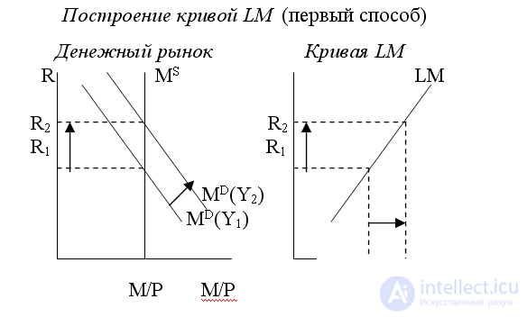
In fig. 3.(a) кривая LM строится на основе графика равновесия денежного рынка (выводимого из кейнсианской теории предпочтения ликвидности). Рост уровня дохода (от Y 1 до Y 2 ) увеличивает спрос на деньги, смещая кривую М D вправо, что увеличивает ставку процента от R 1 до R 2 . Это позволяет построить кривую LM, показывающую, что для обеспечения равновесия денежного рынка более высокому уровню дохода будет соответствовать более высокая ставка процента. Поэтому наклон кривой LM положительный.
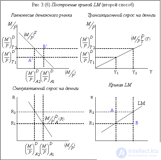
На рис.14.3.(б) кривая LM (IV график) выводится из принципа равенства общего спроса на деньги (включающего: 1) трансакционный спрос на деньги, зависящий от дохода и представленный кривой (M/Р)DT на II графике, и 2) спекулятивный спрос на деньги, зависящий от ставки процента и изображенный кривой (M/Р) D A на III графике) предложению денег (кривая (M/Р) S , представленная на I графике в III квадранте, где показано бюджетное ограничение, налагаемое фиксированным количеством денег в экономике). При уровне дохода Y 1 трансакционный спрос на деньги равен [(M/Р) D T ] 1 , то при существующей в экономике величине предложения денег спекулятивный спрос на деньги составит [(M/P) D A ] 1 , что соответствует ставке процента R 1 . Если уровень дохода возрастет до Y 2 , трансакционный спрос на деньги составит [(M/P) D T ] 2 , при котором спекулятивный спрос на деньги равен [(M/P) D A ] 2 , что соответствует ставке процента R 2 . Таким образом, более высокому уровню дохода соответствует более высокая ставка процента.

Точки вне кривой LM. Все точки, находящиеся вне кривой LM, соответствуют неравновесию денежного рынка. Рассмотрим точку А (рис. 3.(б)), которая находится выше кривой LM. В этой точке уровень дохода равен Y1, что соответствует величине трансакционного спроса на деньги [(M/P) D T ] 1 , а ставка процента составляет R2, что соответствует величине спекулятивного спроса на деньги (M D A ) 2 . Сумма этих величин спросов на деньги соответствует величине предложения денег, характеризуемое точкой A', лежащей на кривой, где предложение денег меньше, чем имеющееся в экономике (кривая (M/P)sup>S). Таким образом, во всех точках, лежащих выше кривой LM, предложение денег превышает общий спрос на деньги, что означают избыточное предложение денег (excess supply of money – ESM). В точке В, которая находится ниже кривой LM трансакционный спрос на деньги составит [(M/P) D T ] 2 , поскольку уровень дохода равен Y 2 , а спекулятивный спрос на деньги равен [(M/P) D A ] 1 , так как ставка процента равна R 1 . Сумма спросов на деньги соответствует величине предложения денег в точке B', где оно меньше, чем имеется в экономике. Таким образом, в этом случае спрос на деньги оказывается выше предложения денег. Следовательно, во всех точках, находящихся ниже кривой LM, имеет место избыточный спрос на деньги (excess demand for money – ESM). Чтобы в этих точках установилось равновесие, необходимо, чтобы либо изменился уровень дохода, либо величина ставки процента, либо и то, и другое. Если снижается ставка процента, то спрос на деньги увеличивается; если снижается уровень дохода, спрос на деньги падает.
Алгебраический анализ кривой LM. Полагая, что функция спроса на деньги линейна, можно получить алгебраическое выражение для кривой LM:
(М/Р) S = kY – hR,
где (М/Р) S – предложение денег, kY – трансакционный спрос на деньги, (- hR) – спекулятивный спрос на деньги. Из этого уравнения получаем значение уровня равновесного дохода:
Y = (1/k)(M/P) S + (h/k)R (1)
и значение равновесной ставки процента:
R = (k/h)Y - (1/h)(M/P) S (2)
Уравнение равновесного дохода дает величину дохода, которая обеспечивает равновесие денежного рынка при любом значении ставки процента и величине реального предложения денег. Аналогично, уравнение равновесной ставки процента показывает величину ставки, которая дает равновесие на рынке денег при любом значении дохода и величине реального предложения денег. Вдоль кривой LM величина реального предложения денег фиксирована.
Поскольку коэффициент при Y в уравнении (2) положительный (k/h > 0, так как k > 0 и h > 0), кривая LM имеет положительный наклон и отражает прямую зависимость между уровнем дохода и ставкой процента. Более высокий доход предопределяет более высокий спрос на деньги, что ведет к более высокой ставке процента.
Сдвиги кривой LM. Сдвиги кривой LM обусловлены изменением номинального предложения денег (М S ). Поскольку уровень цен фиксирован (Р=соnst), то изменение центральным банком количества денег в обращении, меняет реальное предложение денег (М/Р) S . Так как коэффициент при (М/Р) S в уравнении (1) положительный, то рост предложения денег ведет к сдвигу кривой вправо на расстояние ΔМ(1/k), в то время как его сокращение сдвигает кривую на такое же расстояние влево.
Наклон кривой LM. Наклон кривой LM равен (k/h) - коэффициенту, стоящему перед Y в уравнении (2), и зависит от двух параметров: 1) чувствительности спроса на деньги к уровню дохода (k) и 2) чувствительности спроса на деньги к ставке процента (h).
Уменьшение h увеличивает наклон кривой LM (она становится более крутой) и при h = 0 кривая становится вертикальной. При росте h кривая LM становится более пологой. При уменьшении k кривая LM будет более пологой, а при его увеличении – более крутой.
Таким образом, кривая LM будет более пологая, если:
•чувствительность спроса на деньги к изменению ставки процента (h) велика (спрос на деньги чувствителен к изменению ставки процента). Это означает, что даже незначительное изменение ставки процента ведет к существенному изменению спроса на деньги;
•чувствительность спроса на деньги к изменению дохода (k) невелика (спрос на деньги нечувствителен к изменению дохода). Существенное изменение дохода вызывает незначительное изменение спроса на деньги.

Comments
To leave a comment
Macroeconomics
Terms: Macroeconomics