Labor market. Labor supply and demand

Production function

The total supply (output in the economy) is determined by the quantity and quality of available resources. The main economic resources are labor (the amount of time that workers spend on work) and capital (capital (tools of production used by workers in the labor process). The existing technology also has a significant impact on output. The maximum possible output in an economy can be obtained with existing technology and existing stocks of factors of production (potential or natural output) is described by the production function Y = F (K, L, τ) or Y = AF (K, L), where Y is the values and output, K - capital stock, L - labor margin, τ or A - existing technology. The production function has the following properties:

• The output is zero if at least one of the production factors is not used.
• The output increases if the amount of one of the factors increases.
• Increasing the use of one of the factors with a constant amount of another factor leads to a decrease in the return of the first factor, i.e. there is a law of decreasing marginal productivity factors.
• With an increase in the use of one of the factors, the return on the increase in the use of the second factor in production increases.
• With an increase in the number of all factors by x times, the output volume also increases by x times, which means that the production function has constant returns to scale.

All of these properties has the Cobb - Douglas production function, which is most often used in macroeconomics to determine the value of total output. The history of the appearance of this function is as follows. In 1927, the American economist (the future senator from Illinois) Paul Douglas noticed that the distribution of national income between capital and labor almost does not change over time, and workers and owners of capital enjoy equal benefits of economic prosperity. Douglas turned to mathematics Charles Cobb to come up with a function that would describe this phenomenon (the constancy of the shares of production factors in the national income). Cobb showed that these properties will have the function Y = AK ^α L ^1-α , where A is a parameter characterizing the performance of an existing technology, α is a positive parameter, showing the share of income on capital in national income, (1 - α is a positive parameter, showing the share of labor income in national income.

The graph of the production function is presented in Fig. one.

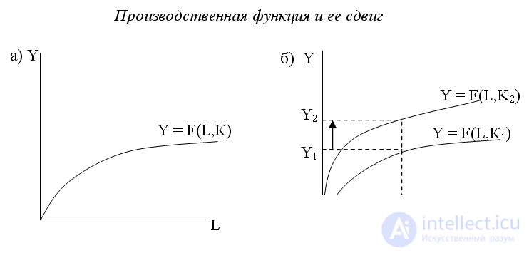
The shift in the production function occurs when the amount of capital changes or technology changes. If the capital stock in the economy increases (from K ₁ to K ₂ ) (Fig. 1. (b)), then the production function shifts up, and with the same amount of labor used (L ₁ ), the total output increases (from Y ₁ to Y ₂ ). Similar changes will occur if more advanced technology is used.

Since in the short term the stock of capital is a constant value and labor is a variable factor, all changes in output are associated with changes in the stock of labor in the economy. Thus, in order to explain changes in output, it is necessary to study the labor market, find out what determines the demand for labor, labor supply and balance in the labor market.

Labor demand

In the labor market, the demand for labor is imposed by firms. The condition for maximizing the profits of firms is the equality of marginal revenue marginal costs (МR = МS). The marginal income of a company from hiring an additional (marginal) worker will be the proceeds from the sale of products produced by this worker, which is equal to the product price of the product (P) and the marginal product of labor (MP _L ), and the marginal costs are the nominal (cash) wage of the worker. So, in order to maximize the company's profit, the following equality must be fulfilled: Р х MP _L = W. The company hires workers, i.e. imposes a demand for labor, so that workers, participating in the production process, create products. Therefore, the firm’s demand for labor is determined by the marginal product of labor or the marginal productivity of labor. The firm’s demand for labor graph is the marginal product (marginal productivity) of labor. Since there is a law of decreasing marginal productivity of labor, the curve has a negative slope.

Thus, the demand for labor is a function of the marginal product of labor: L ^D = L ^D (MP _L ).

From the profit maximization condition: P x MP _L = W, it follows that MP _L = W / P, and since L ^D = L ^D (MP _L ), it follows that L ^D = L ^D (W / P).

This means that the demand for labor is a function of real wages. Moreover, this dependence is negative. The higher the real wage, the lower the demand for labor. A change in real wages leads to movement along the demand curve for labor and to a change in the magnitude of the demand for labor.

Labor supply

Labor supply is carried out by households. When deciding whether or not to work, the household chooses between work (labor) and leisure (doing nothing). In order for a person to refuse to rest and go to work, he must receive, in his opinion, sufficient compensation for this sacrifice. Such compensation is the income received for the labor provided, i.e. wage. A prerequisite for the classic model is that workers have no money illusions. This means that workers never confuse nominal (monetary) wages (W) and real wages (w), i.e. the purchasing power of nominal wages, measured by the ratio of nominal wages to the price level (w = W / P). Therefore, the labor supply in the classical model is a function of the real wage rate: L ^S = L ^S (W / P), and the dependence of the value of the labor supply on the real wage is straight (moving along the curve). A change in nominal wages leads to a shift in the labor supply curve (with a rise in nominal wages, the curve shifts to the right, and when it decreases, to the left).

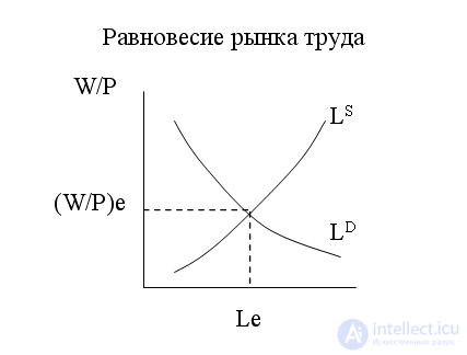
The balance of the labor market is established at the intersection of the demand curve for labor L ^D and the labor supply curve L ^S (Fig. 2.). The equilibrium in the labor market corresponds to the equilibrium real wage rate (W / P) L _e and the equilibrium level of employment (L) _e .

Total offer in the long term

The conditions for the formation of aggregate supply in the short and long term are different. In the long run, the value of aggregate supply is determined by the quantity and quality of the resources available in the economy and the existing technology, so the output does not depend on changes in the price level and other nominal variables; all prices are flexible, prices for resources change in proportion to the change in prices for goods, and the aggregate supply curve is vertical. Therefore, changes in aggregate demand lead only to changes in the price level, while the value of real output remains unchanged (at the level of potential or natural output (natural output), that is, output at full employment of all resources - Y *). This point of view on the aggregate supply curve corresponds to the classical macroeconomic model and describes the behavior of the economy in the long run. We derive the long-term aggregate supply curve graphically (Fig. 1.).

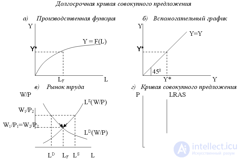
In the classical model, the level of employment is always at its natural level, i.e. at the level of full employment of all labor resources (L _F ). This is explained by the fact that the market always adapts to changes in the situation, prices for resources change in proportion to changes in prices for goods (general price level), and equilibrium is restored, and again at the level of full employment. For example, if the price level decreases from P ₁ to P ₂ , then with the same nominal wage (W ₁ ) the real wage will increase to (W ₁ / P ₂ ). As a result of the increase in real wages, firms will reduce the demand for labor to L ^D , and workers will increase the supply of labor to L ^S. Competition among workers will lead firms to start lowering nominal wages. As a result, real wages will begin to fall, the firm will increase the demand for labor, and the workers will reduce the supply of labor. This will continue until the nominal wage decreases in the same proportion as the general price level and reaches the level W ₂ . With such a nominal wage, the real wage will return to its original level, i.e. W ₁ P ₁ = W ₂ / P ₂ , and the level of employment will again be equal to its natural level LF.

Since the labor market is always in equilibrium (due to the flexibility of nominal wages) and, moreover, at the level of full employment, output will always be equal to the potential output Y * (Fig. 3. (a)), and the aggregate supply curve will be vertical i.e. will not depend on the price level (Fig. 3. (d) and Fig. 3. (a)). Obviously, such a situation is typical for a long-term period, because only in the long-term period is a full market adaptation and proportional change of all prices possible, therefore the vertical aggregate supply curve is a long-term aggregate supply curve (LRAS).

Cumulative offer in the short run

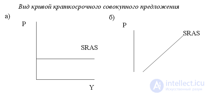
In the short term, prices are rigid, and in the absence of limited resources, the aggregate supply curve has a horizontal view. (Fig. 4. (a)). This is the so-called “extreme Keynesian incident”. This kind of aggregate supply curve justified Keynes, describing the period of the Great Depression of 1929-1933. Since the condition for profit maximization by a firm is equality of marginal revenue, marginal cost (МR = MS), and analysis of the labor market shows that nominal wage rate (W) is the marginal cost for the firm, and marginal revenue for the marginal product, t. e. P x MPL, then the firm will get the maximum profit at W = P x MPL.

If both prices and wages are hard, then MPL = const, i.e. the value is constant, which, as a rule, does not correspond to reality, since the law of decreasing marginal productivity or decreasing marginal product of the factor applies. (However, it should be borne in mind that the Keynes model provides for moderate inflation, i.e. it is only a matter of stiffness of the nominal wage rate, but not of the price stiffness of goods. In this case, the aggregate supply curve has a positive slope.) Therefore, in accordance with modern concepts, the short-term aggregate supply curve has a positive slope (Fig. 4. (b)).

This type of short-term aggregate supply curve is recognized by representatives of both the neoclassical and neo-Keynesian directions, assuming that in the short-term period the aggregate supply depends on the price level and can be represented by the formula proposed by well-known American economist Robert Lucas:

Y = Y * + α (Р - Р ^e )

where Y is the actual output, Y * is the potential output (or the natural level of output), P is the actual price level, P ^e is the expected price level, α is a coefficient showing how much the actual output volume (Y) deviates from its potential level (Y *) when the actual price level (P) deviates from the expected price level (P ^e ).

Thus, the equation shows that actual GDP deviates from its potential level when the actual price level deviates from the expected one. How sensitive the release is to unexpected changes in the price level is shown by the coefficient α. The coefficient α> 0, because if the actual price level exceeds the expected (P ₁ > P ^e ), then the value of the output increases, and the actual GDP will be greater than the potential GDP (Y ₁ > Y *) (point A in Fig. 5.). Conversely, if the actual price level is less than expected (P ₂

e ), the value of output will decrease, and the actual volume of output will become less than the potential (Y ₂

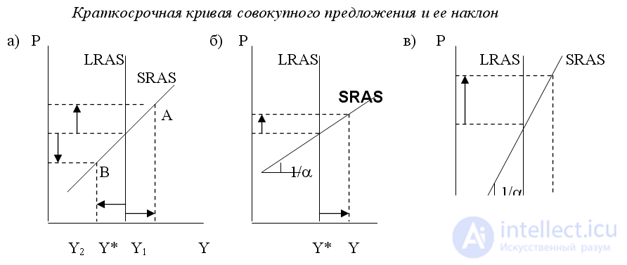
If the coefficient α is small, the short-term aggregate supply curve is steep (the value 1 / α is large). This means that the output is insensitive or weakly sensitive to an unexpected change in the price level, and therefore requires a very significant price shock (increase in the price level from P1 to P2) in order for the actual release to change (Fig. 5. (c)). As R.Lukas showed, who conducted special studies of the sensitivity of output to unexpected changes in the price level in different countries, this is typical for developing countries and countries with transitional economies, who are accustomed to high inflation and frequent and significant unexpected changes in the price level and therefore practically do not react to them. increase in total output.

In different macroeconomic models, the explanations for why the short-term aggregate supply curve has a positive slope are different. There are four explanations (models) for short-term aggregate supply: a rigid nominal wage model, a model of employee misconceptions, an imperfect information model, and a rigid price model.