
Lecture
We classify as electromagnetic those devices in which primary signals about the object or phenomenon under study arise in the form of a change in the magnetic field or in the form of electromagnetic induction signals, and it is precisely these changes or signals that are sensed, analyzed and used to obtain information.
A magnetic field is a force field that acts on physical bodies possessing their own magnetic moment, on moving electric charges and on current-carrying conductors. The magnetic field at each of its points is characterized by the magnetic flux density vector  , whose magnitude is expressed in the SI system in "teslas" (T). Because the atoms, ions and electrons of which a substance is composed have their own magnetic moments, when interacting with a magnetic field they tend to turn in the direction of that field and, as a rule, reinforce it. The amplification coefficient of the magnetic field in a substance is called the "magnetic permeability of the substance". It is a dimensionless quantity and is usually denoted by the Greek letter
  .
.
A number of substances, called "ferromagnets", have a high magnetic permeability ( and higher) because the magnetic moments of the atoms of which they are composed are relatively large. At temperatures below the so-called "Curie point" such spontaneous magnetization becomes "frozen in". So-called "domains" are formed – regions of uniform magnetization which, under the influence of an external magnetic field, are remagnetized as a single whole.
A typical "magnetization curve" of ferromagnetic materials such as iron is shown in fig. 7.1. This is the dependence of the magnetic flux density  inside the ferromagnetic material on the field strength
  of the external magnetic field, created, for example, inside a solenoid. The dashed line marks the so-called "initial magnetization curve". At first
  increases almost linearly with increasing
  . The slope of this section is greater the greater the magnetic permeability of the material
  . However, the rate of increase of
  with increasing
  then decreases, and eventually the magnetic flux density practically ceases to depend on
  . This happens because at such values of
  all the magnetic domains are already oriented in the direction of the external magnetic field. The corresponding value of
  is called the saturation magnetic flux density.
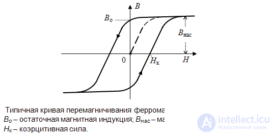
Fig. 7.1.
Further along, the course of the remagnetization curve becomes dependent on the prior history and direction of change of the external magnetic field. When the latter decreases and falls to zero, the ferromagnetic material remains magnetized in the same direction as before. The quantity  is called the remanent magnetization. Under the action of an increasing external magnetic field of the opposite direction, the magnitude of the magnetization decreases to zero, and then the ferromagnet is remagnetized in the new direction. The strength of the external magnetic field
  , at which the magnetic flux density in the ferromagnet becomes equal to zero, is called the coercive force. Overall, the curve of slow remagnetization of a ferromagnet has the form of a closed line symmetric about the origin of coordinates, which is called the "hysteresis loop".
The magnetic field is closely connected with the electric field. The sources of the magnetic field are not only objects with their own magnetic moment, but also moving electric charges and electric current.
A changing magnetic field gives rise to an electric field. In particular, in a closed loop, when the magnetic flux passing through it changes, an electromotive force (EMF) arises and an electric current flows. This phenomenon is called electromagnetic induction. The direction of the induced current is such that the magnetic field it creates opposes the change in magnetic flux through the area of the loop.
Because of the close connection between the magnetic field and the electric field, they are regarded as a single "electromagnetic" field, whose behavior in the classical approximation is described by the well-known Maxwell's equations.
In magnetic sensors the solenoid already mentioned above is often used – a conductor wound into a spiral, through which an electric current flows (fig. 7.2). The magnetic field created inside a current-carrying solenoid is practically uniform, and the magnetic flux density vectors are directed parallel to the axis. The magnetic flux density is proportional to the current strength and the number of turns. Outside the solenoid the configuration of the magnetic field is similar to the configuration of the field of a permanent bar magnet.
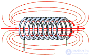
Fig. 7.2. Image of a solenoid and the configuration of its magnetic field
A solenoid with a ferromagnetic core placed inside it becomes an electromagnet, whose force of attraction is proportional to the current strength.
If the electric current through a solenoid changes rapidly, then the magnetic flux passing through it also changes rapidly. Therefore an additional EMF arises in the solenoid ("self-induction EMF"), proportional to the rate of change of the current. The coefficient of proportionality is called the inductance, and the solenoid itself – an "inductor coil". The inductance of a solenoid is fairly large and is proportional to the number of turns in it. The self-induction EMF is directed so as to oppose the change of current in the coil. And in this the phenomenon of self-induction is similar to the phenomenon of inertia in mechanics. Because of this, in alternating electric current circuits the current strength in an inductor coil lags behind the changes in voltage by a quarter period.
If two inductor coils are threaded by a common magnetic flux, a "transformer" is formed. A change of current in one of the coils gives rise to an induced EMF in the other coil – and the greater the number of turns it has, the greater this EMF. The coils can be galvanically decoupled (electrically isolated from one another), with the transfer of electrical energy between them occurring through the common alternating magnetic field. To reduce energy losses caused by the scattering of the magnetic field (i.e. by the fact that some part of the magnetic field lines passes by the other coil), the inductor coils in transformers are connected by a closed magnetic core – a "magnetic circuit", in which practically all the field lines (the entire magnetic flux) are concentrated.
If an inductor coil is electrically connected to a capacitor, an electrical oscillating circuit is formed, in which free electromagnetic oscillations can occur. During such oscillations, the energy stored in the capacitor in the form of electric field energy is periodically transferred into the energy of the magnetic field of the current in the inductor coil, and then – back again. Such a circuit can play the role of an effective frequency filter, which "responds" mainly to electromagnetic oscillations at the "resonant" frequency, i.e. at the frequency of the circuit's own oscillations. This is widely used in electrical engineering and radio engineering, including in the construction of sensors and measuring instruments.
If the electric field lines inside a capacitor or the magnetic field lines inside a solenoid do not close upon themselves, but emerge outward, then part of the oscillation energy is radiated into space in the form of "electromagnetic waves". These can propagate in space at the speed of light over very large distances. Recall that between the propagation velocity  , the frequency
  and the wavelength
  of electromagnetic waves there is a well-known relation:
|
|
(7.1) |
Depending on the oscillation frequency, electromagnetic waves are called radio waves (at frequencies of 103...1012 Hz), infrared radiation (at frequencies of 1012...3.75×1014 Hz), visible light (at frequencies of 3.8...7.5)×1014 Hz, ultraviolet (at frequencies of 7.5×10¹⁴...1016 Hz), X-rays (at frequencies of 1016...1020 Hz) and gamma radiation (at frequencies >1020 Hz).
Radio waves, in turn, are divided by wavelength into bands:
long waves (LW, wavelength 1...10 km, corresponding frequency 300...30 kHz);
medium waves (MW, wavelength 100...1000 m, frequency 3...0.3 MHz);
short waves (SW, wavelength 10...100 m, frequency 30...3 MHz);
ultrashort or metre waves (VHF, wavelength 1...10 m, frequency 300...30 MHz, engl. VHF - Very High Frequency);
decimetre waves (engl. UHF - Ultra High Frequency, wavelength 1...10 dm, frequency 3000...300 MHz);
centimetre waves (wavelength 1...10 cm, frequency 30...3 GHz);
millimetre waves (wavelength 1...10 mm, frequency 300...30 GHz).
The character of radio wave propagation in the Earth's atmosphere depends substantially on the band. While long and medium waves easily follow the curvature of the Earth's surface and are therefore received by radio receivers practically at any point on the globe, the propagation of short and especially ultrashort waves depends substantially on the state of the troposphere. Decimetre and centimetre waves are received mainly only within line of sight.
Both the mechanical and the magnetic properties of iron, steel, cast-iron and other products made from ferromagnetic materials are directly determined by their microcrystalline structure. Therefore, by measuring their magnetic properties – magnetic permeability, coercive force, saturation magnetic flux density, etc. – it is possible to monitor compliance with the manufacturing process regimes, the microstructure and the mechanical properties.
Well-known magnetic sensors are magnetic reading heads,– for reading data from other magnetic information carriers (from magnetic tapes, disks, drums, cards, etc.). Magnetic reading heads always deal at their input with signals, with information encoded in the form of a varying magnetic field on the surface of the carrier.
Self-check questions 7 .
Which sensors belong to the electromagnetic class?
Name the main radio wave bands.
What is magnetic diagnostics?


Comments