Lecture
So far, we have considered physical systems whose various states  it was possible to list everything; the probabilities of these states were some nonzero magnitudes
  . Such systems are similar to discontinuous (discrete) random variables, taking values
  with probabilities
  . In practice, physical systems of a different type are often encountered, similar to continuous random variables. The states of such systems cannot be renumbered: they continuously go from one to another, with each individual state having a probability equal to zero, and the probability distribution is characterized by a certain density. Such systems, by analogy with continuous random variables, we will call "continuous", in contrast to the previously considered, which we will call "discrete". The simplest example of a continuous system is a system whose state is described by one continuous random variable.
  with distribution density
  . In more complex cases, the state of the system is described by several random variables.
  with distribution density
  . Then it can be considered as an association.
  simple systems
  .
.
Consider a simple system.  defined by one continuous random variable
  with distribution density
  (fig. 18.7.1). We will try to extend to this system entered in
  18.1 the concept of entropy.
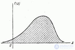
Fig. 18.7.1.
First of all, we note that the concept of a “continuous system,” like the concept of a “continuous random variable,” is a kind of idealization. For example, when we consider the value  - growth at random taken by a person - a continuous random variable, we are distracted from the fact that no one actually measures growth more precisely than 1 cm, and that it is almost impossible to distinguish between two growth values that differ, say, by 1 mm. Nevertheless, it is natural to describe this random variable as continuous, although it could be described as discrete, considering those values that differ by less than 1 cm to coincide.
Similarly, by setting the limit of measurement accuracy, i.e., some segment  within which the system state
  practically indistinguishable, you can approximate a continuous system
  to discrete. This is equivalent to replacing a smooth curve.
  step type histogram (Fig. 18.7.2); at the same time each section (discharge) of length
  replaced by one representative point.
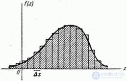
Fig. 18.7.2.
The squares of the rectangles represent the probabilities of hitting the corresponding bits:  . If we agree to consider indistinguishable system states belonging to the same category, and combine them all into one state, then we can approximately determine the entropy of the system
  considered up to
  :
:

 . (18.7.1)
When small enough  :
:
 ,
,

and the formula (18.7.1) takes the form:
 . (18.7.2)
Note that in expression (18.7.2), the first term turned out to be completely independent of  - the degree of accuracy in determining system states. Depends on
  only second member
  which tends to infinity when
  . This is natural, since the more precisely we want to set the state of the system
  , the greater degree of uncertainty we need to eliminate, and with unlimited reduction
  this uncertainty grows unlimited too.
So, asking an arbitrarily small "insensitivity area"  our measuring instruments, which determine the state of the physical system
  entropy can be found
  by the formula (18.7.2), in which the second term grows indefinitely with decreasing
  . Entropy itself
  differs from this unlimitedly growing member by independent of
  magnitude
 . (18.7.3)
This value can be called the “reduced entropy” of a continuous system.  . Entropy
  expressed through reduced entropy
  by formula
 . (18.7.4)
The ratio (18.7.4) can be interpreted as follows: on the measurement accuracy  depends only on the origin, at which the entropy is calculated.
In the future, to simplify the record, we will omit the index  in the designation of entropy and write just
  ; Availability
  the right side will always indicate the accuracy of which.
Formula (18.7.2) for entropy can be given a more compact form, if, as we did for discontinuous quantities, we write it in the form of the mathematical expectation of a function. First of all, we rewrite (18.7.2) as
 . (18.7.5)
This is nothing more than the expectation of a function.  from random variable
  with density
  :
:
 . (18.7.6)
A similar form can be given to  :
:
 . (18.7.7)
Let us proceed to the definition of conditional entropy. Suppose there are two continuous systems:  and
and  . In general, these systems are dependent. Denote
  distribution density for states of the combined system
  ;
;  - system distribution density
  ;
;  - system distribution density
  ;
;  - conditional density of distribution.
First, we define the partial conditional entropy.  i.e. system entropy
  provided that the system
  took a certain state
  . The formula for it will be similar (18.4.2), only instead of conditional probabilities
  there will be conditional distribution laws
  and a term will appear
  :
:
 . (18.7.8)
We now turn to the full (average) conditional entropy  , for this you need to average private conditional entropy
  in all states
  taking into account their probabilities, characterized by a density
  :
:
 (18.7.9)
or, considering that
 ,
,
 . (18.7.10)
Otherwise, this formula can be written as
 (18.7.11)
or
 . (18.7.12)
Having thus determined the conditional entropy, let us show how it is used in determining the entropy of the combined system.
We first find the entropy of the combined system directly. If “dead spots” for systems  and
and  will be
  and
and  then for a unified system
  the elementary rectangle will play their role
  . Entropy system
  will be
 . (18.7.13)
Because
 ,
,
then and
 . (18.7.14)
Let's substitute (18.7.14) in (18.7.13):

 ,
,
or, according to the formulas (18.7.6) and (18.7.12)
 , (18.7.15)
that is, the entropy theorem of a complex system also holds for continuous systems.
If a  and
and  are independent, the entropy of the combined system is equal to the sum of the entropies of the constituent parts:
 . (18.7.16)
Example 1. Find the entropy of a continuous system  , which all states on some site
  equally likely:

Decision.
 ;
;

or
 . (18.7.17)
Example 2. Find the entropy of the system  The states of which are distributed according to the normal law:
 .
.
Decision.

 .
.
But
 ,
,

and
 . (18.7.18)
Example 3. The condition of the aircraft is characterized by three random variables: height  , speed module
  and angle
  determining the direction of flight. The height of the aircraft is distributed with a uniform density on the site
  ; speed
  - under the normal law with m.
  and s.ko.
  ; angle
  - with uniform density on the site
  . Values
  are independent. Find the entropy of the combined system.
Decision.
From example 1 (formula (18.7.17)) we have
 ,
,
Where  - “deadband” when determining the height.
Так как энтропия случайной величины не зависит от ее математического ожидания, то для определения энтропии величины  воспользуемся формулой (18.7.18):
 .
.
Энтропия величины  :
:
 .
.
Finally we have:

or
 . (18.7.19)
Заметим, что каждый из сомножителей под знаком фигурной скобки имеет один и тот же смысл: он показывает, сколько «участков нечувствительности» укладывается в некотором характерном для данной случайной величины отрезке. В случае распределения с равномерной плотностью этот участок представляет собой просто участок возможных значений случайной величины; в случае нормального распределения этот участок равен  where
where  - среднее квадратическое отклонение.
Таким образом, мы распространили понятие энтропии на случай непрерывных систем. Аналогично может быть распространено и понятие информации. При этом неопределенность, связанная с наличием в выражении энтропии неограниченно возрастающего слагаемого, отпадает: при вычислении информации, как разности двух энтропий, эти члены взаимно уничтожаются. Поэтому все виды информации, связанные с непрерывными величинами, оказываются не зависящими от «участка нечувствительности»  .
.
Выражение для полной взаимной информации, содержащейся в двух непрерывных системах  and
and  , будет аналогично выражению (18.5.4), но с заменой вероятностей законами распределения, а сумм - интегралами:
 (18.7.20)
или, применяя знак математического ожидания,
 . (18.7.21)
Полная взаимная информация  как и в случае дискретных систем, есть неотрицательная величина, обращающаяся в нуль только тогда, когда системы
  and
and  are independent.
Пример 4. На отрезке  выбираются случайным образом, независимо друг от друга, две точки
  and
and  , каждая из них распределена на этом отрезке с равномерной плотностью. В результате опыта одна из точек легла правее, другая - левее. Сколько информации о положении правой точки дает значение положения левой?
Decision. Рассмотрим две случайные точки  and
and  на оси абсцисс
  (рис. 18.7.3).

Fig. 18.7.3.
Denote  абсциссу той из них, которая оказалась слева, а
  - абсциссу той, которая оказалась справа (на рис. 18.7.3 слева оказалась точка
  , но могло быть и наоборот). Values
  and
and  определяются через
  and
and  следующим образом
 ;
;  .
.
Найдем закон распределения системы  . Because
  , it will exist only in the region
  shaded in fig. 18.7.4.
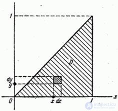
Fig. 18.7.4.
Denote  the distribution density of the system
  and find the element of probability
  , that is, the probability that a random point
  falls into an elementary rectangle
 .This event can occur in two ways: either there is a dot on the left and a dot
  on the right
  , or vice versa. Consequently,
 ,
,
Where  marked density distribution of the system of values
  .
.
In this case

 ,
,
Consequently,
 ;
;

and

We now find the laws of the distribution of individual quantities in the system:
 at
at  ;
;
similarly
 at
at  .
.
Density graphs  and
and  shown in fig. 18.7.5.
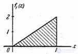
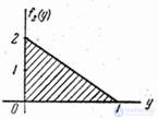
Figure 18.7.5.
Substituting  ,
,  and
and  in the formula (18.7.20), we get

 .
.
By virtue of the symmetry of the problem, the last two integrals are equal, and

 (two units).
Example 5. There is a random variable  distributed according to the normal law with parameters
 ,
,  . Magnitude
  измеряется с ошибкой
  , тоже распределенной по нормальному закону с параметрами
  ,
,  . Mistake
  does not depend on
  . В нашем распоряжении - результат измерения, т. е. случайная величина

Определить, сколько информации о величине  содержит величина
  .
.
Decision. Воспользуемся для вычисления информации формулой (18.7.21), т. е. найдем ее как математическое ожидание случайной величины
 . (18.7.22)
Для этого сначала преобразуем выражение
 .
.
In our case
 ,
,
 (см. главу 9).
Выражение (18.7.22) равно:

 .
.
From here
 . (18.7.23)
Ho  , Consequently,
 (18.7.24)
Подставляя (18.7.24) в (18.7.23), получим
 (two units).
For example, when 
 (two units).
If a  ;
;  then
then  (two units).
Comments
To leave a comment
Information and Coding Theory
Terms: Information and Coding Theory