
Lecture
Robotic manipulators.
The use of manipulators became commonplace as far back as the 20th century. Today, no major industrial production can do without them. In addition, manipulators are also fitted to mobile robots to extend control capabilities in places that are hard for a person to reach. For repetitive and monotonous tasks, a robot can also replace a human — for example, arranging pastries into boxes. So, let us define a manipulator as a controlled device designed to perform complex actions similar to the movements of a human arm. This also includes a mechanism for controlling the position of objects.
Manipulator arm
To master manipulator control, you should go back to controlling motor position using a P-controller, which was described
in the chapter "Control Algorithms." Only the design will differ somewhat from the one described (fig. 8.148-8.149).
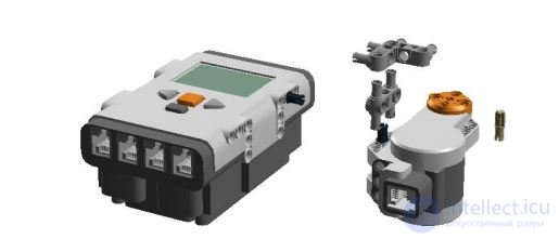
Fig. 8.148. Mounting the motor to the NXT body horizontally at surface level. The pin-axle is inserted into the motor shaft from below.
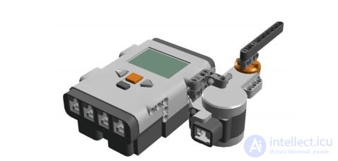
Fig. 8.149. First joint of the manipulator.
The manipulator arm is positioned horizontally. The control algorithm consists of two parallel tasks. In the first, a
P-controller runs, holding the motor at position alpha. In the second, the value of alpha changes over time (fig. 8.150).
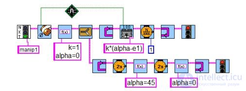
Fig. 8.150. Controlling the horizontal position of the manipulator arm.
Given that the zero position is set at startup, set a negative angle in the second parallel task and perform a
sequential transition through zero. If everything works, proceed to installing the second motor with the gripper.
Manipulator with a gripper
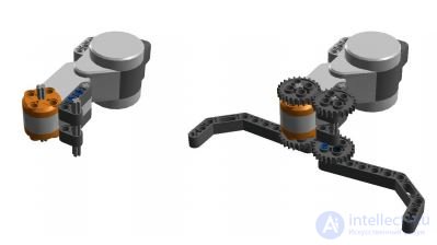
Fig. 8.151. Mounting the gripper on the second motor.
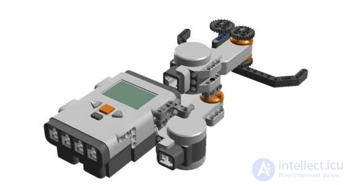
Fig. 8.152. The motor with the gripper is mounted on the disk of the first motor.
Fig. 8.152. The motor with the gripper is mounted on the disk of the first motor.
Programming a robot with two degrees of freedom (fig. 8.151-8.152) is done similarly. A new variable beta will
define the position of the second motor. Extend the second task by selecting suitable values for opening and closing the gripper
(fig. 8.153). Remember that the starting position determines everything.
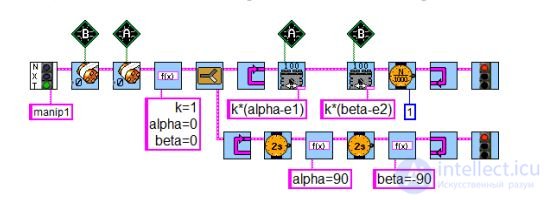
Fig. 8.153. A template for controlling two motors based on P-controllers. The loop in the parallel task needs to be continued.
Precise positioning. Discrete controller.
Bibliographic description: Musaev G. M. Modeling of the positioning system of a solar energy concentrator reflector [Text] / G. M. Musaev // Molodoy Uchenyi (Young Scientist). — 2013. — No. 3. — pp. 81-83.
The goal of creating a precise angular positioning system is to develop and manufacture the hardware and software needed to provide computer-based control of a positioning system for various objects. Direct current motors with gearboxes and angular displacement sensors of various types are used as the actuator.
Solving scientific and practical problems requires ensuring angular positioning of objects with high precision .
The main parameters of the system include:
Accuracy of coordinate determination.
Positioning accuracy.
Control systems for dynamic objects with digital controllers represent a fairly complex class to describe. The continuous part of the system (the controlled plant) is defined by differential equations, whereas the microprocessors implementing the control device algorithms are represented by difference equations. A mixed description in the form of differential and difference equations, supplemented by relations for analog-to-digital and digital-to-analog converters, creates significant difficulties in solving typical analysis and synthesis problems. Therefore, in control practice, models that describe the behavior of systems only at discrete (clock) instants of time have become widespread. This makes it possible to limit the description to difference equations alone, which radically simplifies the description of the systems under consideration and the solution of the corresponding controller synthesis problems.
An alternative approach, by contrast, proposes limiting the initial description of the system to differential equations and synthesizing continuous controllers, which are then implemented on microprocessors only after synthesis. Both of these approaches are widely used in control practice, although each of them has its own methodological errors.
An alternative approach to the synthesis of discrete controllers proposes solving control problems while remaining within the framework of continuous systems. In this case, a continuous controller is synthesized, which is then implemented using digital methods. It is physically clear that the behavior of a discrete system will approach the behavior of a continuous one as the sampling period decreases. To evaluate the changes introduced into the dynamics of continuous systems by the use of microprocessors, let us first consider the frequency characteristics of the zero-order extrapolator
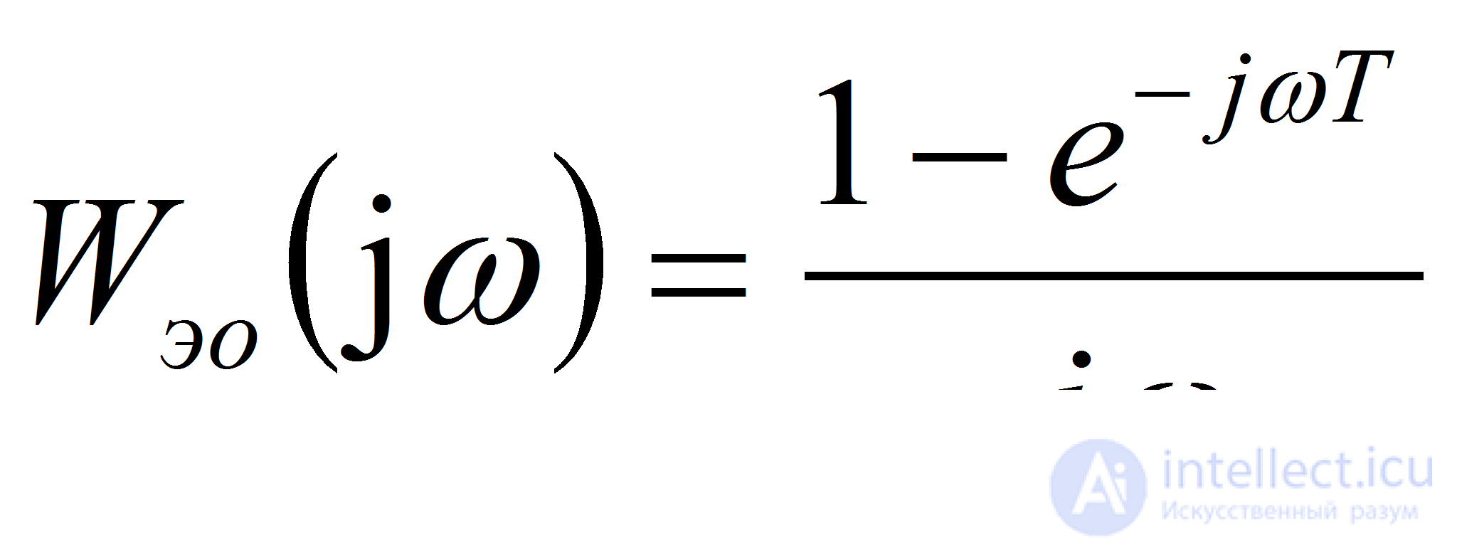 (1)
(1)
Replacing the exponential with trigonometric functions, after simple transformations we find
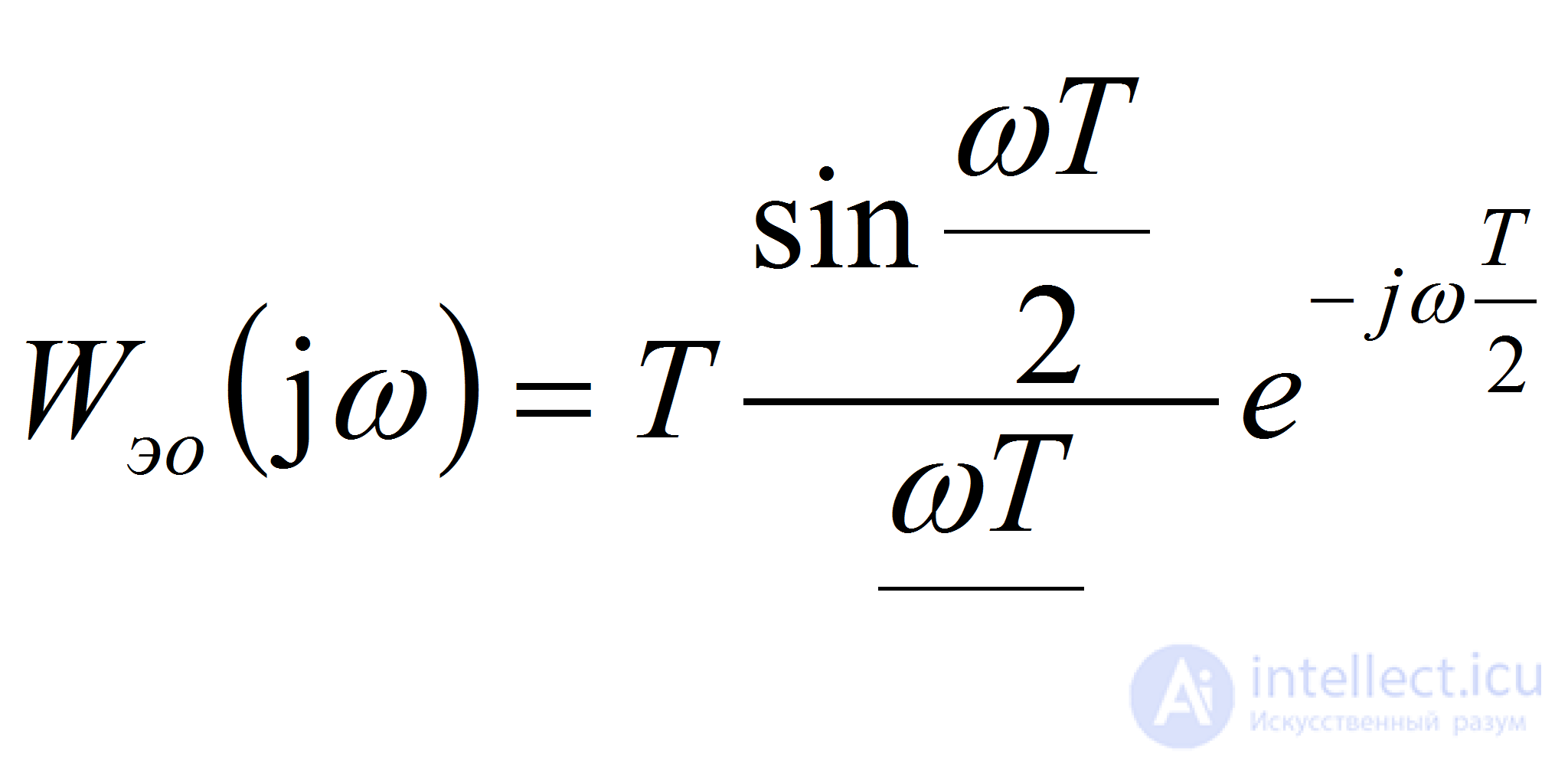 (2)
(2)
From the last relation it is evident that the gain of the extrapolator is equal to the sampling period. The extrapolator introduces a pure delay equal to half the sampling period. When designing, the sampling frequency is chosen to be significantly greater than the range of the system's operating frequencies.
Converters introduce an additional delay into the system, equal to half the sampling period. Therefore, when controllers are subsequently implemented on a microprocessor, their synthesis should be carried out for a modified plant that differs from the original one by the presence of a pure delay element
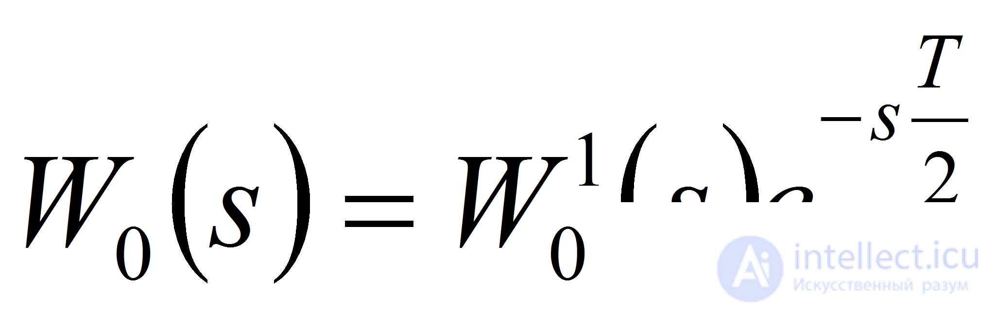 (3)
(3)
As an example of a control system for a dynamic object with digital controllers, let us consider a control device for a direct current motor. DC motors are used in drives that require smooth control of rotational speed over a wide range.
The main component of the DC motor control device, which acts as the converter and source of control signals, can be a microcontroller (MCU).
The properties of DC motors are determined by their starting, operating, mechanical, and control characteristics.
The subscripts "B" and "A" denote the parameters and variables of the field and armature circuits; L — inductance, R — resistance, U — voltage, i — current; M — electromagnetic torque of the motor, e — armature EMF.
The motor used in servo systems is required to convert an electrical signal (control voltage) into an armature rotation speed proportional to the magnitude of the signal. As a rule, DC motors with independent (separate) field excitation are used. A schematic diagram of the motor is shown in fig. 1.
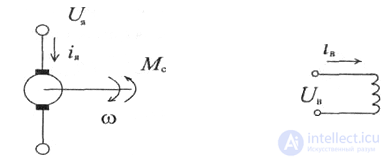
Fig. 1. Schematic diagram of a DC motor.
The motor can be controlled by varying the voltage either in the armature circuit UA, or in the control winding circuit UB..
Let us first consider the static equations. The armature circuit current /A, the field excitation magnetic flux ΦB, the torque Mrot, the rotational speed of the motor shaft ω and the back-EMF ep,induced in the armature winding, are related by the following equations:
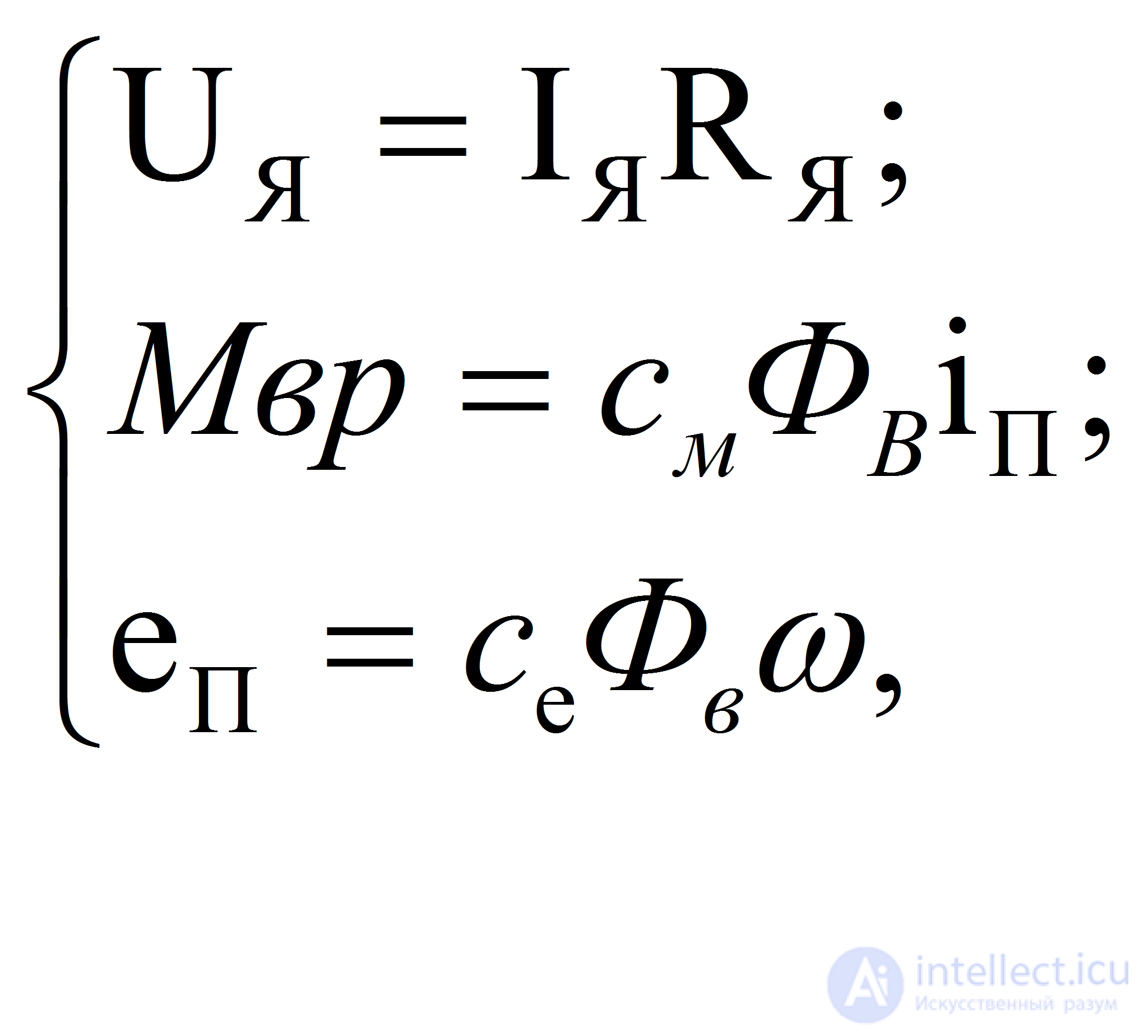 (4)
(4)
where 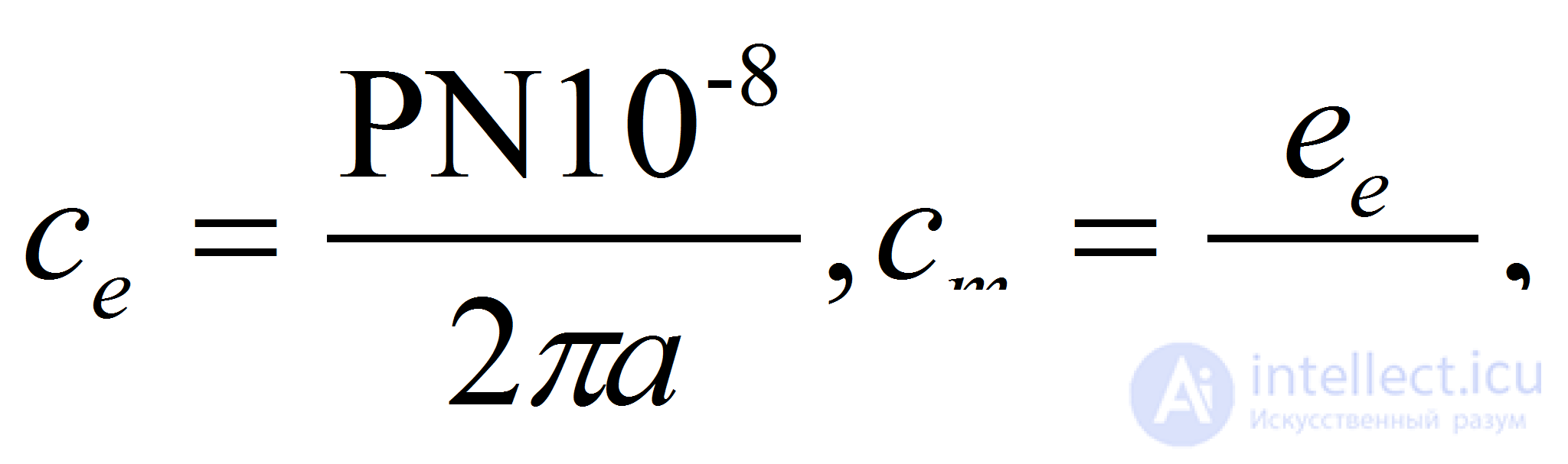
N — number of armature conductors, P — number of pole pairs, a — number of parallel branch pairs, RA — resistance of the armature circuit. Excluding ep and iA from the equation, we obtain
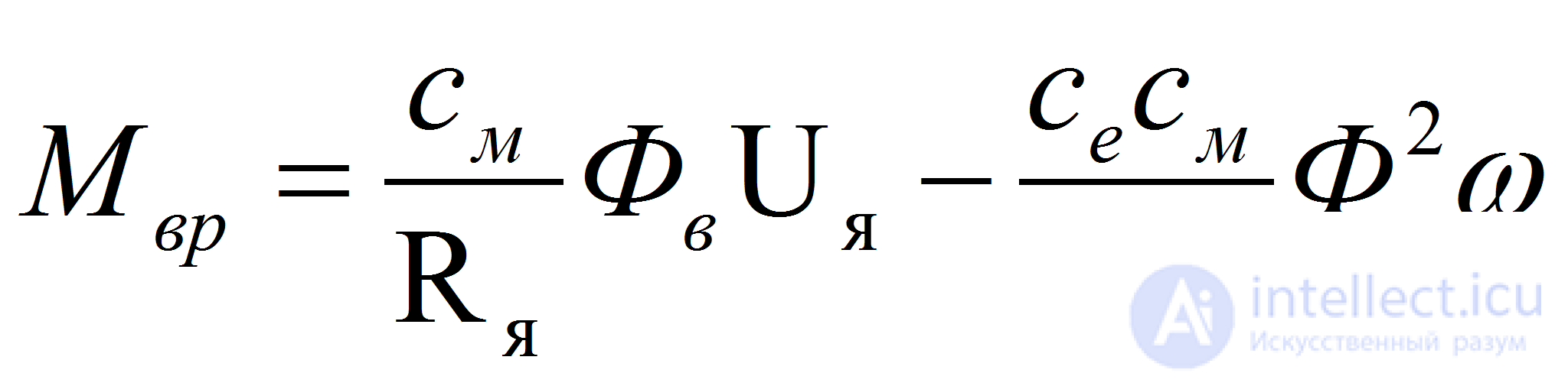 (5)
(5)
From formula (4), which defines the motor's mechanical characteristic, it is evident that with a constant field flux ΦB, produced by a fixed field voltage UB,the torque depends linearly on the control signal in the armature circuit UA. This makes it possible to smoothly vary the motor speed over a wide range. Because of this, in the servo system under consideration, motor control is carried out specifically through the armature circuit. Let us formulate the dynamics equation for a DC motor controlled through the armature circuit.
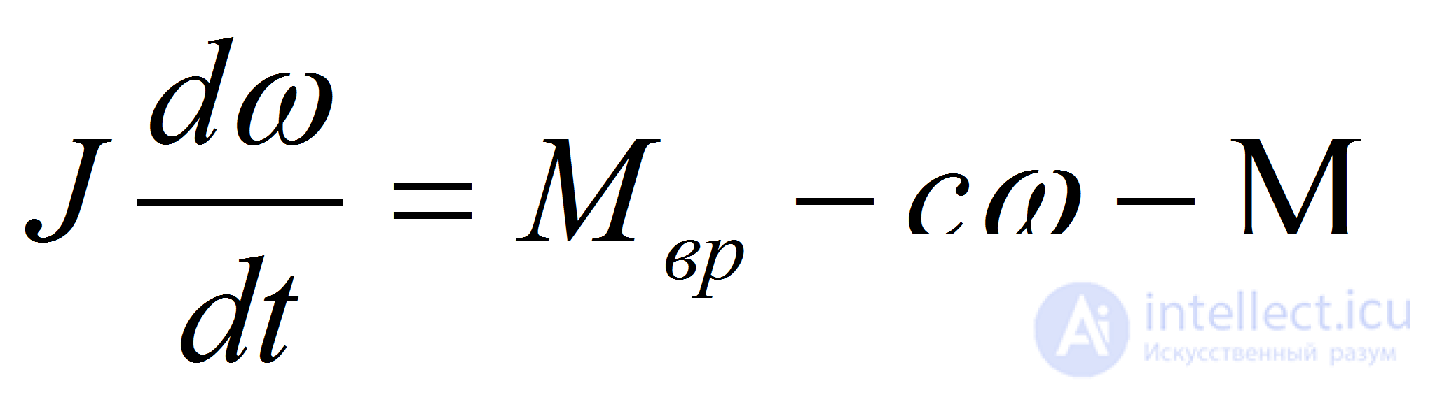
The equation of motion of the motor armature has the form
 (6)
(6)
Here J — moment of inertia of all rotating masses reduced to the motor shaft, c —viscous friction coefficient, Mc — load torque.
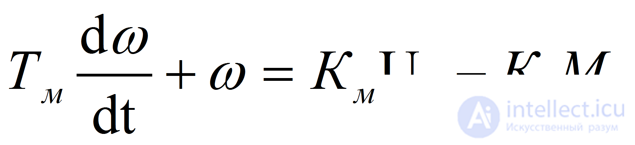
From (5) and (6) we obtain

or
 (7)
(7)
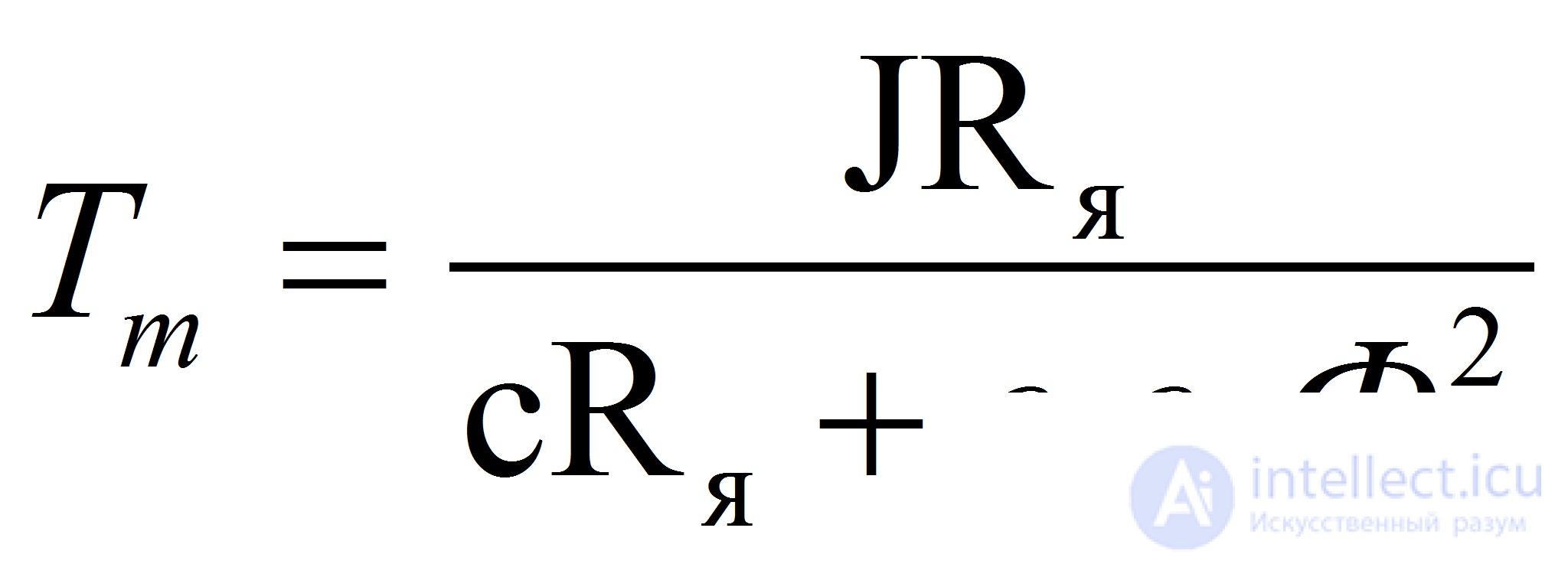
where Tm — is the motor time constant, Km — is the motor's control-input gain, Kc— is the motor's disturbance-input gain:
 ;
; 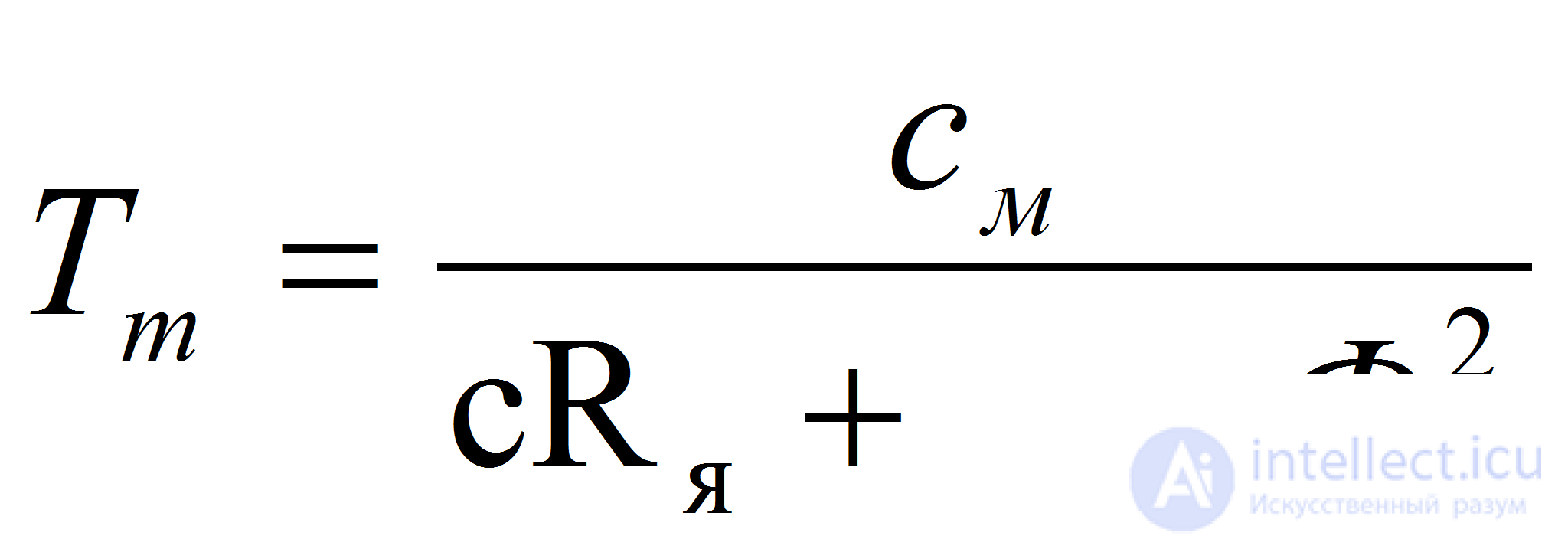 ;
; 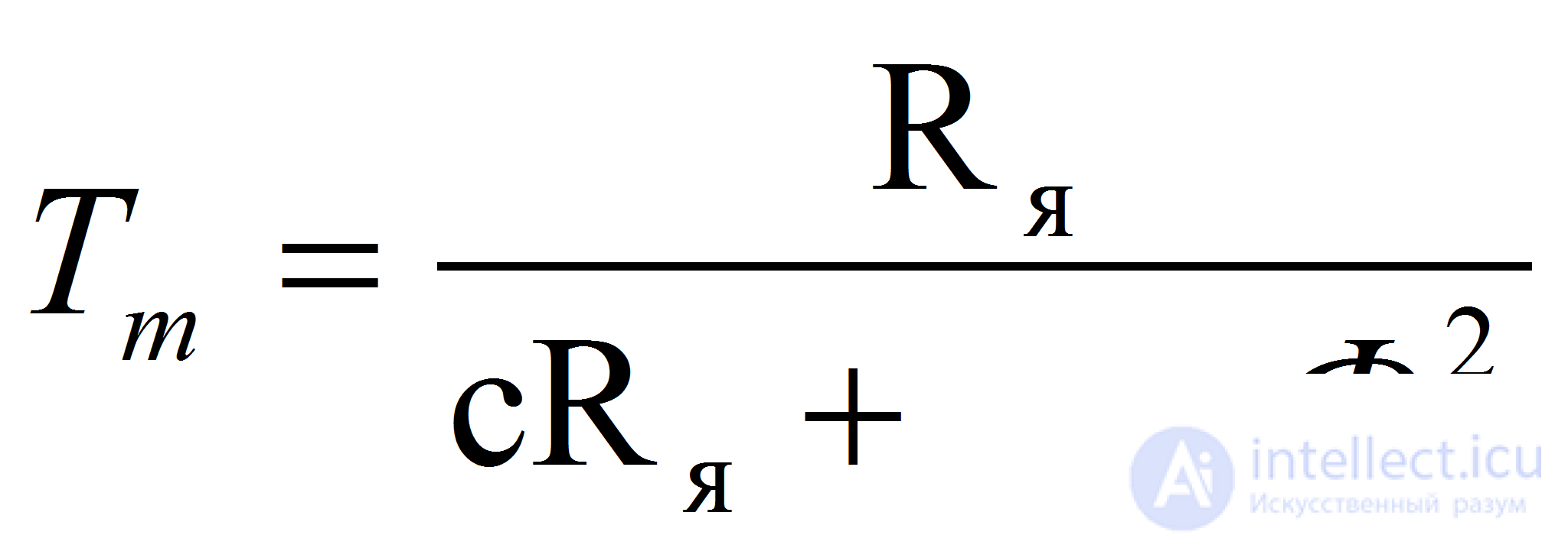 (8)
(8)
Accordingly, the motor's transfer functions with respect to the control input and the disturbance (load torque), relative to angular velocity, have the form
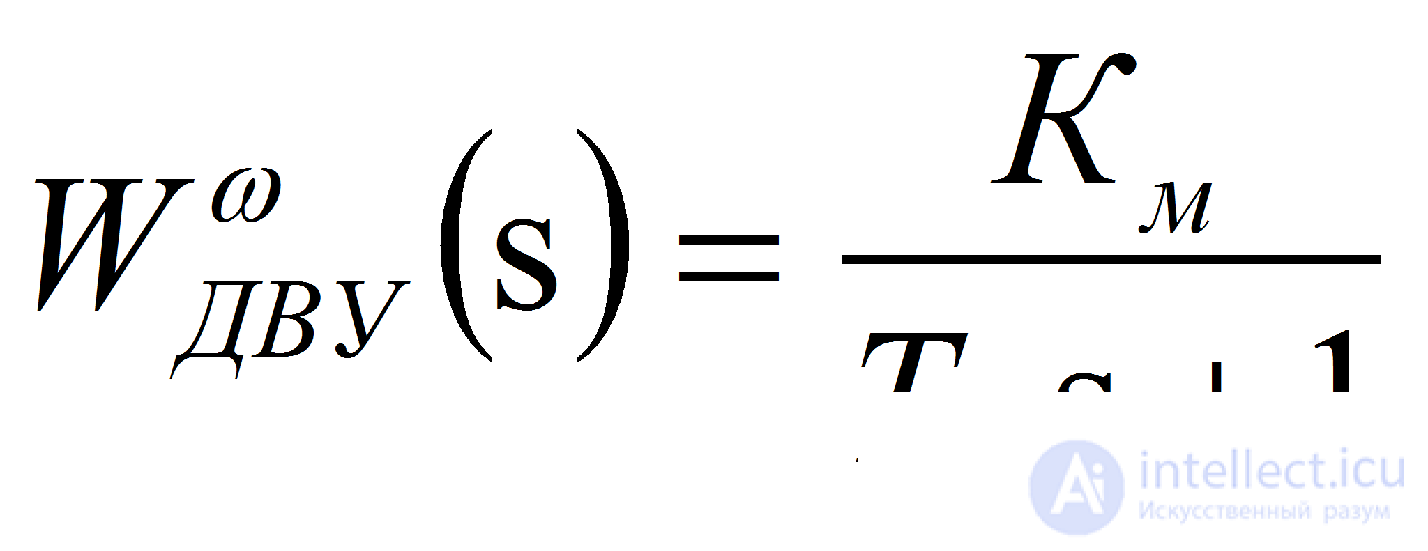 ;
; 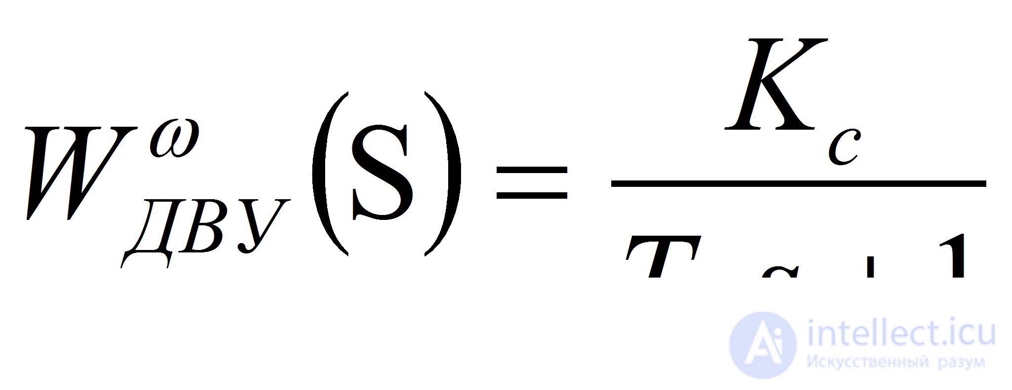 (9)
(9)
Equation (7) can be written with respect to the rotation angle. Given that 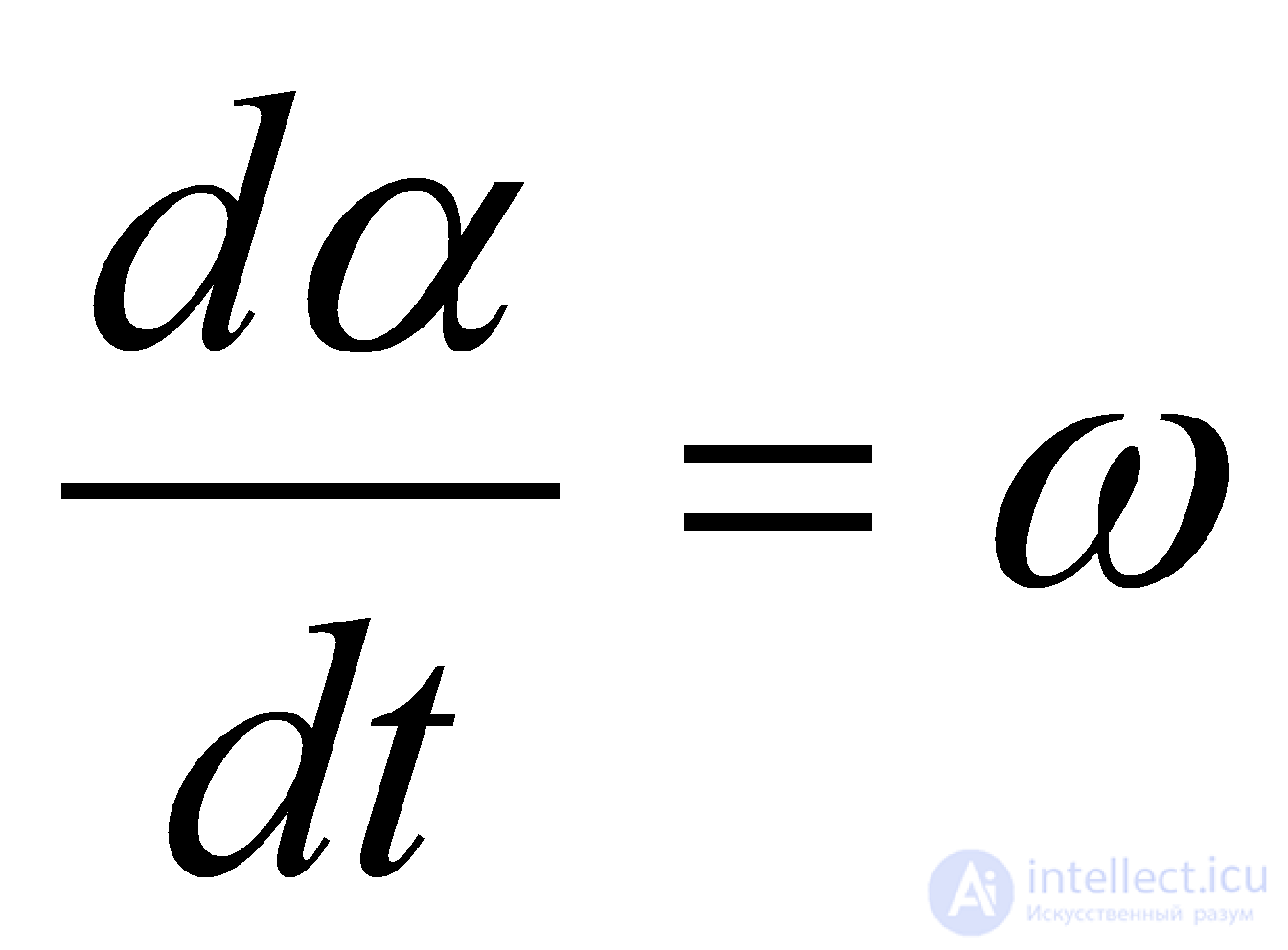 we obtain the following equation:
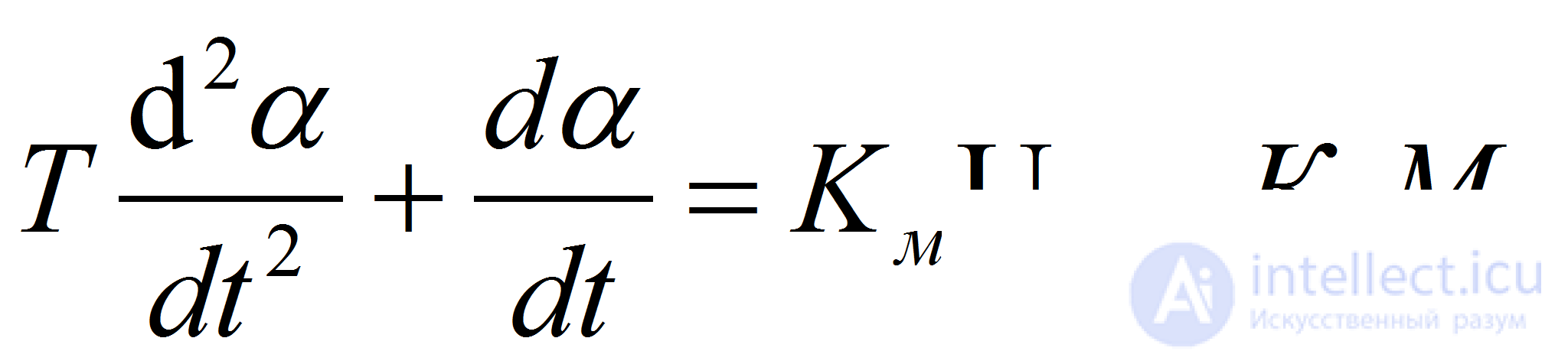 (10)
(10)
The motor described by equation (11) has two corresponding transfer functions — with respect to the control input and with respect to the disturbance, relative to the rotation angle:
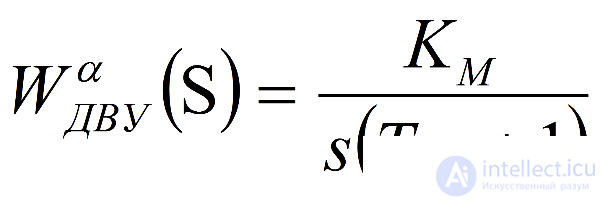 (11)
(11)
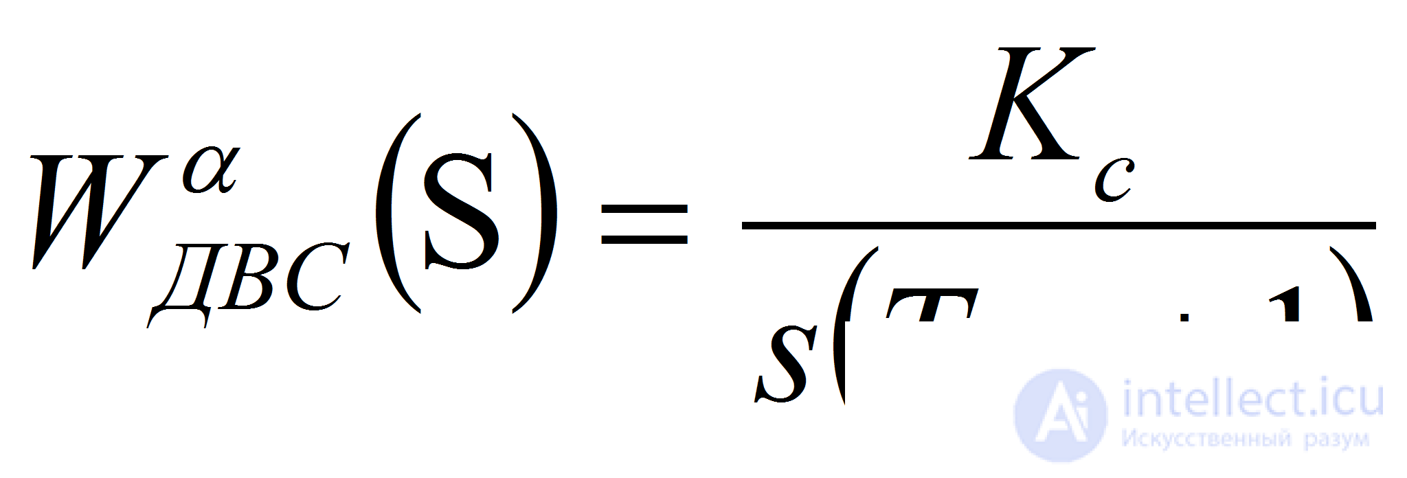 (12)
(12)

Comments