Proportional-derivative controller.

PID controller

Diagram illustrating the operating principle of a PID controller. The coefficients in front of the integral and derivative terms are omitted for clarity.

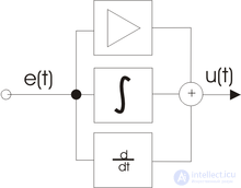
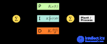
A proportional-integral-derivative (PID) controller is a device in a closed-loop control system. It is used in automatic control systems to form a control signal in order to achieve the required accuracy and quality of the transient process. A PID controller forms a control signal that is the sum of three terms, the first of which is proportional to the difference between the input signal and the feedback signal (the error signal), the second is the integral of the error signal, and the third is the derivative of the error signal.

If some of the components are not used, the controller is called a proportional-integral, proportional-derivative, or proportional controller, and so on.

General information

Proportional term

The proportional term produces an output signal that counteracts the deviation of the controlled variable from the setpoint observed at the current moment. The larger the deviation, the larger this term is. If the input signal equals the setpoint, the output is zero.

However, when using only a proportional controller, the value of the controlled variable never stabilizes exactly at the setpoint. There is a so-called steady-state error, equal to the deviation of the controlled variable that produces an output signal stabilizing the output variable at that particular value. For example, in a temperature controller the output signal (heater power) gradually decreases as the temperature approaches the setpoint, and the system stabilizes when the power equals the heat losses. The temperature cannot reach the setpoint, because at that point the heater power would become zero and the heater would start cooling down.

The larger the proportionality coefficient between the input and output signals (the gain), the smaller the steady-state error; however, with too large a gain, and in the presence of delays in the system, self-oscillations may begin, and with a further increase in the gain the system may become unstable.

Integral term

The integral term is proportional to the integral of the deviation of the controlled variable. It is used to eliminate the steady-state error. It allows the controller to account for the steady-state error over time.

If the system experiences no external disturbances, then after some time the controlled variable stabilizes at the setpoint, the signal of the proportional term becomes zero, and the output signal is provided entirely by the integral term. Nevertheless, the integral term can also lead to self-oscillations.

Derivative term

The derivative term is proportional to the rate of change of the deviation of the controlled variable and is intended to counteract deviations from the target value that are predicted to occur in the future. Such deviations may be caused by external disturbances or by a delay in the controller's effect on the system.

Theory

The output signal of the controller u is determined by three terms: the purpose of the PID controller is to maintain a given value x₀ of some quantity x by adjusting another quantity u. The value x₀ is called the setpoint (or set value, in engineering), and the difference e = (x₀ − x) is called the residual (or [control] error, in engineering), the mismatch, or the deviation of the quantity from the setpoint.

,

where K_p, K_i, K_d are the gain coefficients of the proportional, integral, and derivative terms of the controller, respectively.

Most PID tuning methods use a somewhat different formula for the output signal, in which the integral and derivative terms are also multiplied by the proportional gain:

In a discrete implementation of the output-signal calculation method, the equation takes the following form:

,

where is the sampling time. Using the substitution we can write:

In software implementations, to optimize the calculations one switches to the recurrent formula:

A closed-loop control system involving a PID controller. The system controls the quantity y(t), i.e. it drives the quantity y(t) to an externally given value u(t). The error e(t) is fed to the input of the PID controller, and the output of the PID controller is the control action for some process (the plant), which governs the quantity y(t).

The following are often used as parameters of a PID controller:

• relative range

• integration and derivative time constants, which have the dimension of time

It should be noted that these terms are used differently in different sources and by different controller manufacturers.

References

• How PID controllers work
• Implementing a PID controller in C++
• Translation of the article "PID algorithms made simple"

Isn't the program given as an exercise for understanding NXT-G in this post similar to the programs explaining line following in this one?




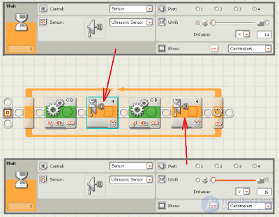
The difference between the programs is that one uses a distance sensor, while the other uses a light sensor. Otherwise the programs are similar: the robot changes its turning direction after the sensor reading changes.

To be more precise, in the task the robot turns right if the sensor's distance reading is less than 14 cm, and left if the distance reading is greater than 16 cm. It's hard to imagine why such motion would be needed if the sensor points forward or backward. But a lot falls into place if we assume that the sensor is mounted on one of the robot's sides and points sideways.



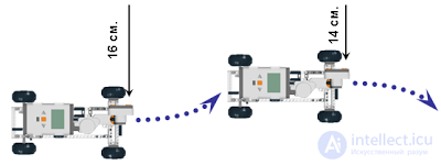
If you draw a diagram of such motion, it becomes clear that there is some obstacle along the robot's left side throughout the motion, and the robot is trying not to drive too close to it and not to move too far away from it. If we assume that the obstacle is a wall, the robot's motion can be called wall following. On gentle bends of the wall, the robot will try to keep a certain distance, i.e. it will turn along with the bend of the wall.



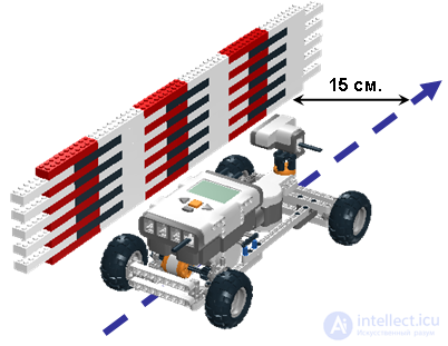
By the way, this answer (wall following) was also among the answers that were sent in after the task was published.

As with the proposed line-following algorithm, it should be kept in mind that this implementation of wall following is also a basic one for study purposes. That is, in real-world tasks the motion algorithm will be significantly more complex, but the underlying principle of motion remains the same.

Now we'd like to draw attention to one detail that those who are just starting to implement wall following quite often "trip over."

In general, the robot moves parallel to the wall, and the distance sensor shows the expected value, based on which a decision is made about which way to turn.

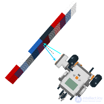
But a situation can arise where the robot, in trying to get closer to the wall again, turns significantly toward it. This causes the sensor to start reading a very large distance - the signal reflected off the wall no longer reaches the sensor, and it "thinks" that the obstacle is still too far away.

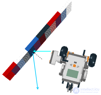
In this case, the robot will try to get closer to the wall, increasing the angle between the sensor and the wall, which will only make the situation worse.

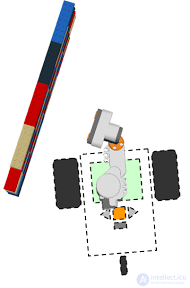
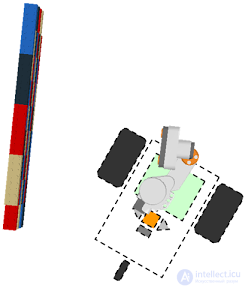
There isn't just one traditional solution to this problem. It can be either a software solution or a design solution. For example, instead of mounting the sensor rigidly, you can mount it on a motor.

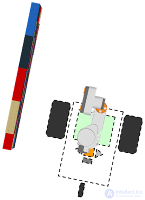
This way, after the robot turns, say, left, the distance sensor turns, trying to stay pointed directly at the wall. And when turning right, the motor turns the sensor the other way:

This scheme is especially convenient when building a robot with a steering motor, since in that case the sensor can be mounted on the same motor that controls the steering wheels. It is better to mount it not directly, but by selecting a suitable gear combination.

5.1.7. Wall following

Let's solve the following task. The robot must move along a wall at a given distance L. Suppose the robot's left wheel is driven by motor B, the right wheel by motor C, and the distance sensor, connected to port 1, is mounted slightly ahead of the cart's body (this is important!) and points at the wall to the right of the direction of travel.

Fig. 5.6.

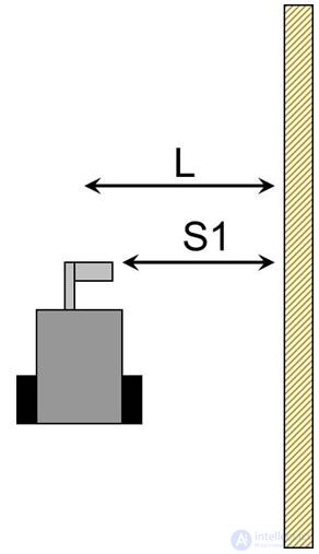
Let us denote the current distance to the wall shown by the sensor as .

The motors move at an average speed of 50, but when deviating from the set course a control action up is applied to them. Let us denote this as follows.

    Motor[MotorB]=50+up;
    Motor[MotorC]=50-up;
    

It remains to determine what the control action will be equal to. This is easy:

Thus, when the robot does not change course and drives straight. If there is a deviation, its course is corrected. Here is some gain coefficient that determines the controller's effect on the system. For a medium-sized NXT robot the coefficient k can range from 1 to 10 depending on many factors. We suggest determining it yourself.

In this case, the controller will work effectively only for small deviation angles. In addition, the motion will almost always follow a wavy trajectory. Introducing new principles that account for the robot's deviation from course will make the control more precise.

5.1.8. Proportional-derivative controller

Fig. 5.7.

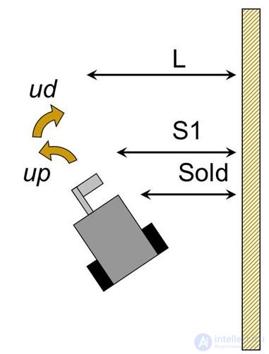
In some situations a P-controller can push the system out of a stable state. For example, if the robot is pointed away from the wall but is closer to it than the set distance, the motors will receive a command to turn even further away from the wall, which may result in losing contact with it (recall that the distance sensor receives a reflected signal reliably only from a perpendicular surface).

Fig. 5.8.

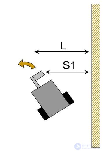
To guard against such situations, let's add a derivative term to the controller that will track the direction of the robot's motion. In other words, the velocity vector will influence the control action. It is known that velocity is found as , where is the change in distance over the time interval . Let us define the derivative controller through the rate of the robot's deviation from the set position:

where is the current distance to the wall, and is the distance at the previous step.

Since measurements are taken at equal time intervals, can be treated as a constant.

Thus, the PD controller is described by a formula with two terms

It can be shown that for stable convergence to the goal, the coefficient of the derivative term must exceed (see the article "Elements of automatic control theory in school" below).

The wall-following algorithm using a PD controller will generally look like this:

Sold=L=S1;
    while(true)
    {
    upd= k1*(S1-L) + k2*(S1-Sold);

    Motor[MotorB]=50+upd;
    Motor[MotorC]=50-upd;

    Sold=S1;
    wait1msec(1);
    }
    

To go around obstacles, it is necessary to introduce monitoring of the distance sensor readings: on a sharp change, the robot must conclude that a turn is possibly occurring, which will need to be performed with different coefficients.