
Lecture 28 min.
Hard disk request scheduling algorithms are an important part of operating systems and file systems. They determine the order in which requests to read or write data on disk are processed, so as to minimize access time and optimize the performance of the I/O subsystem.
Before moving on to the algorithms themselves, let us recall the internal design of a hard disk drive and determine which request parameters we can use for scheduling.
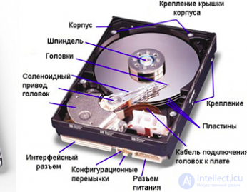
When evaluating hard disk drive performance, the most important characteristic is the data transfer rate. At the same time, a whole range of factors affects speed and overall performance:
But if we take two hard disk drives of the same capacity and the same interface, the key performance factor will be the spindle rotation speed.
The spindle is the single axis in a hard disk drive on which several magnetic platters are mounted. These platters are fixed to the spindle at a strictly defined distance. The distance must be such that, as the platters rotate, the read heads can read from and write to the disk without touching the surface of the platters.
For the drive to function properly, the spindle motor must provide stable rotation of the magnetic platters over thousands of hours. It is therefore not surprising that problems with a drive are sometimes caused precisely by a seized spindle and not at all by file system errors.
The motor is responsible for rotating the platters, and this is what allows the hard disk drive to work.
The spindle rotation speed (spindle speed) determines how fast the platters rotate during normal hard disk drive operation. The rotation speed is measured in revolutions per minute (RpM).
The rotation speed determines how quickly the computer can obtain data from the hard disk drive. Before the drive can read data, it must first find it.
The time required for the magnetic head assembly to move to the requested track/cylinder is called the seek time (seek latency). After the read heads have moved to the required track/cylinder, one has to wait for the platters to turn so that the required sector comes under the head. This is called rotational latency time and is a direct function of the spindle speed. That is, the faster the spindle speed, the lower the rotational latency.
The combined seek time and rotational latency determine the data access speed. In many programs for evaluating HDD speed this is the access to data time parameter.
Most standard 3.5″ hard disk drives today have a spindle rotation speed of 7200 revolutions per minute. For such drives the time taken for half a revolution (avg. rotational latency) is 4.2 ms. The average seek time of these drives is about 8.5 ms, which makes it possible to access data in approximately 12.7 ms.
WD Raptor hard disk drives have a magnetic platter rotation speed of 10,000 revolutions per minute. This reduces the average rotational latency to 3 ms. The "Raptors" also have smaller-diameter platters, which made it possible to cut the average seek time to ~5.5 ms. The resulting average data access time is approximately 8.5 ms.
There are several SCSI models (for example, the Seagate Cheetah) whose spindle rotation speed reaches 15,000 revolutions per minute and whose platters are even smaller than those of the WD Raptor. Their average rotational latency is 2 ms (60 sec / 15,000 RPM / 2), their average seek time is 3.8 ms, and their average data access time is 5.8 ms.
Drives with a high spindle rotation speed have low values of both seek time and rotational latency (even with random access). Clearly, hard disk drives with spindle speeds of 5600 and 7200 offer lower performance.
At the same time, with sequential access to data in large blocks the difference will be insignificant, since there is no data access delay. For this reason it is recommended that hard disk drives be defragmented regularly.
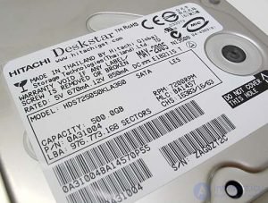
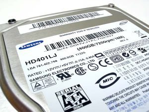
On some models the spindle speed is written directly on the label. This information is easy to find, since there are not many options — 5400, 7200 or 10,000 RpM.
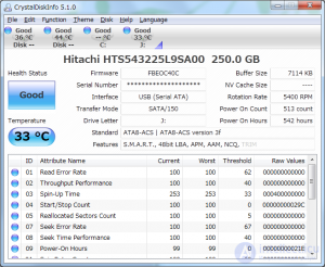
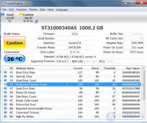
If the label on your hard disk drive does not carry this information (or you simply do not feel like taking the drive out to look at the label), special programs will come to the rescue. Most programs for checking an HDD and analyzing SMART will show you the spindle rotation speed and other information about the hard disk drive.
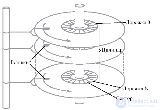
A modern hard magnetic disk is a set of round platters located on a single axis and coated on one or both sides with a special magnetic layer (see Fig. 13.2). Near each working surface of each platter are magnetic heads for reading and writing information. These heads are attached to a special arm that can move the entire head assembly over the platter surfaces as a single unit. The platter surfaces are divided into concentric rings, inside which information can actually be stored. The set of concentric rings on all platters for one position of the heads (i.e., all rings equidistant from the axis) forms a cylinder. Each ring within a cylinder is called a track (one or two tracks per platter). All tracks are divided into an equal number of sectors. The number of tracks, cylinders and sectors can vary within fairly wide limits from one hard disk drive to another. As a rule, the sector is the minimum amount of information that can be read from the disk at one time.
While the drive operates, the set of platters rotates about its axis at high speed, bringing all the sectors of the corresponding tracks under the heads in turn. The sector number, the track number and the cylinder number uniquely determine the location of data on the hard disk and, together with the type of operation performed – read or write – fully characterize the device-related part of a request when information is exchanged in the amount of one sector.
When scheduling the use of a hard disk drive, the natural scheduling parameter is the time that will be required to service the next request. The time needed to read or write a particular sector on a particular track of a particular cylinder can be divided into two components: the time for exchanging information between the magnetic head and the computer, which usually does not depend on the location of the data and is determined by the transfer speed, and the time needed to position the head over the given sector – the positioning time. The positioning time, in turn, consists of the time needed to move the heads to the required cylinder – the seek time – and the time required for the required sector to turn under the head – the rotational latency. Seek times are proportional to the difference between the cylinder numbers of the previous and the planned requests, and they are easy to compare. Rotational latency is determined by rather complex relationships between the cylinder and sector numbers of the previous and the planned requests and the speeds of disk rotation and head movement. Without knowing the ratio of these speeds, comparison becomes impossible. It is therefore natural that the set of scheduling parameters is reduced to the seek times of the various requests, determined by the current position of the head and the numbers of the required cylinders, while the difference in rotational latencies is neglected.
Disk scheduling is performed by operating systems to schedule the I/O requests arriving at the disk. Disk scheduling is also known as I/O scheduling.
Disk scheduling is important because:
There are many disk scheduling algorithms, but before discussing them let us briefly review some of the important terms:
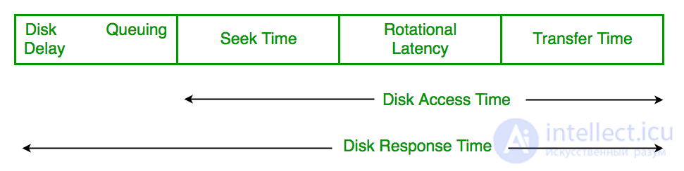 Disk response time: response time is the average time spent by a request waiting to perform its I/O operation. Average response time is the response time of all requests. Variance response time is a measure of how an individual request is serviced relative to the average response time. Thus, a disk scheduling algorithm that gives the minimum variance response time is better
The simplest algorithm, one we should already be used to, is First Come First Served (FCFS) – first come, first served. All requests are organized into a FIFO queue and serviced in order of arrival. The algorithm is simple to implement, but can lead to a fairly long overall request servicing time. Let us consider an example. Suppose that on a disk of 100 cylinders (from 0 to 99) we have the following request queue: 23, 67, 55, 14, 31, 7, 84, 10, and the heads are initially on cylinder 63. Then the position of the heads will change as follows:
63->23->67->55->14->31->7->84->10
and in total the heads travel across 329 cylinders.
(63-23)+(67-23)+(67-55)+(55-14)+(31-14)+(31-7)+(84-7)+(84-10) =329
The inefficiency of the algorithm is well illustrated by the last two movements: from cylinder 7 across the whole disk to cylinder 84, and then back across the whole disk to cylinder 10. Simply swapping the order of the last two movements (7  10 84) would substantially reduce the total time needed to service the requests. So let us move on to another algorithm.
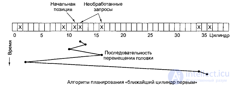
As we have seen, it is quite reasonable to service first those requests whose data lies near the current head position, and only then the ones that are far away. The Short Seek Time First (SSTF) algorithm is based on exactly this idea. For each next service step we select the request whose data lies closest to the current position of the magnetic heads. Naturally, when there are equidistant requests, the choice between them may be made on various grounds, for example according to the FCFS algorithm. For the previous example the algorithm gives the following sequence of head positions:
63->67->55->31->23->14->10->7->84
and in total the heads travel across 141 cylinders. Note that our algorithm resembles the SJF algorithm for process scheduling, if the distance between the current head position and the position required to satisfy a request is taken as the analog of the estimated next CPU burst of a process. And exactly like the SJF algorithm, it can lead to some request being postponed for a very long time. It should be remembered that requests can appear in the queue at any moment. If all our requests but one are constantly clustered in the region of high cylinder numbers, that single request may stay in the queue indefinitely.
The exact SJF algorithm was optimal for a given set of processes with given CPU burst times. Clearly, the SSTF algorithm is not optimal. If we move the servicing of the request for cylinder 67 into the interval between the requests for cylinders 7 and 84, we reduce the total service time. This observation leads us to the idea of a whole family of other algorithms - the scanning algorithms.
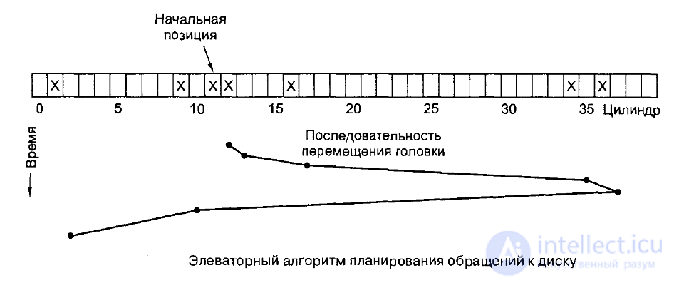
In the simplest of the scanning algorithms - SCAN - the heads move continuously from one edge of the disk to the other, servicing along the way every request they encounter. On reaching the other edge the direction of motion is reversed, and everything repeats again. Suppose that in the previous example the heads are initially moving in the direction of decreasing cylinder numbers. Then we obtain the request service order that we glimpsed at the end of the previous section. The sequence of head movements looks as follows:
63->55->31->23->14->10->7->0->67->84
and in total the heads travel across 147 cylinders.
If we know that we have serviced the last request lying ahead in the direction of head motion, then we need not travel all the way to the edge of the disk and can reverse the direction of motion immediately:
63->55->31->23->14->10->7->67->84
and in total the heads travel across 133 cylinders. This modification of the SCAN algorithm is called LOOK.
Suppose that by the time the direction of head motion is reversed in the SCAN algorithm, that is, when the head has reached one of the edges of the disk, a large number of new requests has accumulated near that edge, and servicing them will take quite a lot of time (let us not forget that the head must not only be moved, but the data read must also be transferred!). Then requests that belong to the other edge of the disk and arrived earlier will wait for service unfairly long. To reduce the waiting time of requests, another modification of the SCAN algorithm is used - circular scanning. When the head reaches one of the edges of the disk, it moves to the other edge without reading the requests along the way (sometimes considerably faster than during an ordinary cylinder seek), and from there it again starts moving in the same direction as before. For this algorithm, called C-SCAN, the sequence of movements looks like this:
63->55->31->23->14->10->7->0->99->84->67
By analogy with the LOOK algorithm for the SCAN algorithm, a C-LOOK algorithm can also be proposed for the C-SCAN algorithm:
63->55->31->23->14->10->7->84->67
There are other varieties of scanning algorithms, and entirely different algorithms as well, but we shall stop here, for it has been said: "And once again I say: no one can embrace the unembraceable".
Let us consider an example. Suppose that on a disk of 28 cylinders (from 0 to 27) we have the following queue of requests:
27, 2, 26, 3, 19, 0
and the heads are initially on cylinder 1. Then the head position will change as follows:
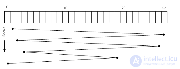
The FCFS algorithm
As can be seen, the algorithm is not very impressive, but it is simple to implement.
For the previous example the algorithm gives the following sequence of head positions:
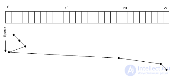
The SSF algorithm
As we can see, this algorithm is more efficient. But it has a drawback: if new requests keep arriving constantly, the head will always stay in one local area, most likely in the middle part of the disk, and the outermost cylinders may never be serviced.
The algorithm is more efficient, but it has a drawback: if new requests keep arriving constantly, the head will always stay in one local area, most likely in the middle part of the disk, and those at the edge of the boundary may never be detected.
The SCAN algorithm - the heads move continuously from one edge of the disk to the other, servicing along the way every request they encounter. Simple, but not always efficient.
Suppose the requests to be addressed are: -82,170,43,140,24,16,190. And the read/write arm is at 50, and it is also given that the disk arm must move "toward the larger value".
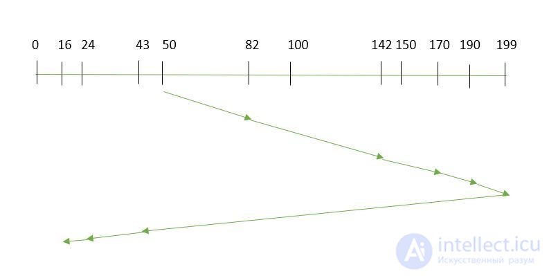
Therefore, the seek time is calculated as:= (199-50) + (199-16)
= 332
Advantages:
Disadvantages:
The LOOK algorithm - if it is known that the last request lying ahead in the direction of head motion has been serviced, then the head need not travel all the way to the edge of the disk and can reverse its direction of motion immediately.
CLOOK: since LOOK is similar to the SCAN algorithm, CLOOK is likewise similar to the CSCAN disk scheduling algorithm. In CLOOK the disk arm, instead of going all the way to the end, goes only as far as the last request to be serviced in front of the head, and then from there jumps to the last request at the other end. In this way it also avoids the extra delay that arose from the unnecessary trip to the end of the disk.
Suppose the requests to be addressed are: -82,170,43,140,24,16,190. And the read/write arm is at 50, and it is also given that the disk arm must move "toward the larger value".
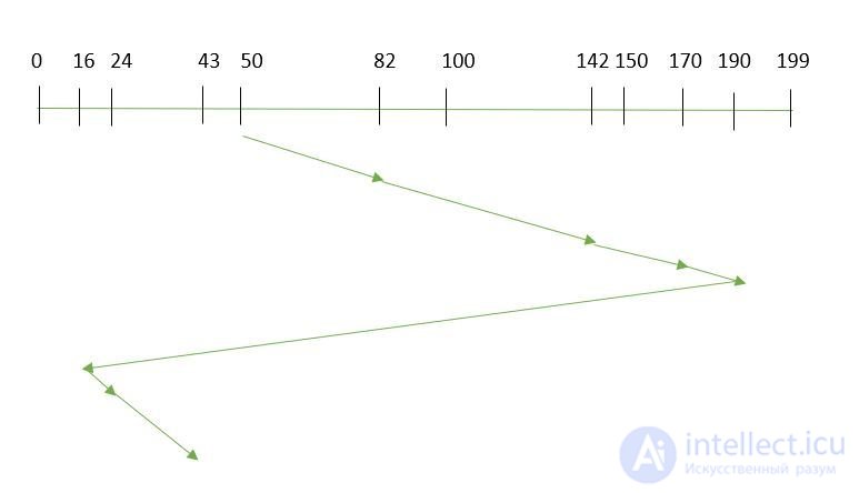
So the seek time is calculated as:
= (190-50) + (190-16) + (43-16)
= 341
Given an array of track numbers on a disk and the initial head position, our task is to find the total number of seek operations performed to access all the requested tracks if the C-LOOK disk scheduling algorithm is used. In addition, write a program to find the seek sequence using the C-LOOK disk scheduling algorithm.
C-LOOK (Circular LOOK) disk scheduling algorithm:
C-LOOK is an improved version of both the SCAN and the LOOK scheduling algorithms. This algorithm also uses the idea of wrapping the tracks around in the form of a circular cylinder, like the C-SCAN algorithm, but the seek time is better than in the C-SCAN algorithm. We know that C-SCAN is used to avoid starvation and services all requests more uniformly; the same applies to C-LOOK.
In this algorithm the head services requests in one direction only (left or right) until all requests in that direction have been serviced, and then it jumps back to the farthest request in the other direction and services the remaining requests, which gives better uniformity of service and also avoids wasting time seeking all the way to the end of the disk.
The algorithm -
Let the Request array be an array that stores the indices of the tracks that have been requested, in ascending order of their arrival times, and let head be the position of the disk head.
The initial direction in which the head moves is given, and it services in that same direction.
The head services all the requests one by one in the direction in which it is moving.
The head keeps moving in the same direction until all the requests in that direction have been serviced.
While moving in this direction, calculate the absolute distance of the tracks from the head.
Increment the total seek count by this distance.
The position of the track currently being serviced now becomes the new head position.
Go to step 5 until we reach the last request in this direction.
If we reach the last request in the current direction, then reverse the direction and move the head in that direction until we reach the last request that needs to be serviced in that direction, without servicing the intermediate requests.
Reverse the direction and go to step 3 until all the requests have been processed.
Examples:
Input:
request sequence = {176, 79, 34, 60, 92, 11, 41, 114}
Initial head position = 50
Direction = right (moving from left to right)
Output:
Initial head position: 50
Total number of seek operations = 156
Seek sequence
60
79
92
114
176
11
34
41
The following table shows the order in which the requested tracks are serviced using C-LOOK.
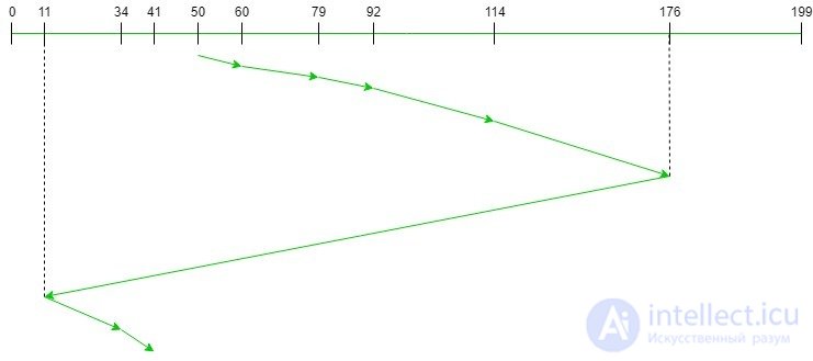
Thus, the total number of seeks = (60-50) + (79-60) + (92-79) + (114-92) + (176-114) + (176-11) + (34-11) + ( 41 - 34) = 321
The C-SCAN algorithm is circular scanning: when the head reaches one of the edges of the disk, it moves to cylinder zero without reading any requests along the way, and from there it begins moving again.
Given an array of track numbers on the disk and the initial position of the head, our task is to find the total number of seek operations performed in accessing all of the requested tracks when the C-SCAN disk scheduling algorithm is used.
What is the C-SCAN (Circular Elevator) disk scheduling algorithm?
The circular scan (C-SCAN) scheduling algorithm is a modified version of the SCAN disk scheduling algorithm that removes the inefficiency of SCAN by servicing requests more uniformly. Like SCAN (the elevator algorithm), C-SCAN moves the head from one end, servicing all requests, to the other end. However, as soon as the head reaches the other end, it immediately returns to the beginning of the disk without servicing any requests on the way back (see the diagram below), and starts servicing again as soon as it reaches the beginning. This is also known as the "circular elevator algorithm", because it essentially treats the cylinders as a circular list that wraps around from the last cylinder to the first.
Algorithm:
Examples:
Input: Request sequence = {176, 79, 34, 60, 92, 11, 41, 114} Initial head position = 50 Output: Initial head position: 50 Total number of seek operations = 190 Seek sequence 60 79 92 114 176 199 0 11 34 41
The following diagram shows the order in which the requested tracks are serviced using SCAN.
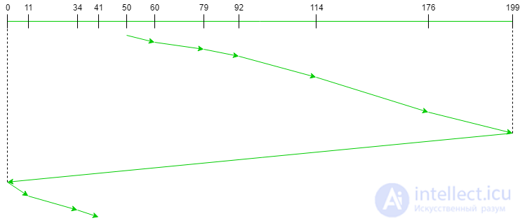
Consequently, the total number of seeks is calculated as:
= (60-50) + (79-60) + (92-79)
+ (114-92) + (176-114) + (199-176) + (199-0)
+ (11-0) + (34-11) + (41-34)
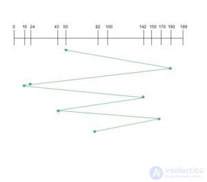
The RSS algorithm - this stands for random scheduling, and, as its name suggests, that is its nature. It is used in situations where the scheduling involves random attributes such as random processing times, random due dates, random weights and stochastic machine breakdowns; for these this algorithm is ideal. That is why it is normally used for analysis and modeling.
Advantages
Disadvantages
Example
Suppose the order of the requests is (82,170,43,142,24,16,190),
and the current position of the read/write head is 50
Advantages
Each algorithm is unique in its own way. Overall performance depends on the number and the type of requests.
Note. The average rotational latency is usually taken to be 1/2 (the rotational latency).
Thus, we have looked at several classic algorithms for scheduling requests to a hard disk:
First-Come, First-Served (FCFS): This is a simple algorithm in which requests are processed in the order in which they arrive. However, it can lead to the problem of "starvation", where some requests wait a long time because new requests keep arriving.
Shortest Seek Time First (SSTF): This algorithm selects the request that has the smallest distance to the disk head. It is aimed at minimizing the travel time of the disk head. However, it too has a problem: requests located at the edges of the disk can be forgotten, which can lead to the so-called "forgotten request" effect (the "forgetful read" problem).
SCAN (Elevator) Algorithm: The disk head moves from one end to the other and processes all requests along its way. When it reaches the end, it reverses direction. This method is efficient, but it can cause delays for requests located in the middle of the disk.
C-SCAN (Circular SCAN) Algorithm: Similar to the SCAN algorithm, but on reaching the far boundary of the disk the head returns to the starting boundary, minimizing the time delays for requests.
LOOK Algorithm: Similar to SCAN, but on reaching the edge of the disk the head changes direction without stopping. This reduces delays compared with SCAN.
C-LOOK Algorithm: A combination of C-SCAN and LOOK. The head moves in one direction only, passing through all of the requests, and then returns to the starting boundary.
The choice of a particular algorithm depends on the performance requirements, the data structures and the specifics of how the hard disk is used in a given system. Some modern operating systems and file systems may use combinations of these algorithms, or improvements on them, to manage requests to the hard disk more efficiently.

Comments