Sample (Empirical) Distribution Function with Examples

Lecture

The sample (empirical) distribution function in mathematical statistics is an approximation of the theoretical distribution function, constructed using a sample drawn from it.

Definition

Let Sample (Empirical) Distribution Function with Examples be a sample of size , generated by a random variable , given by the distribution function . We will assume that , where , are independent random variables defined on some sample space of elementary outcomes . Let . Define the function as follows:

Sample (Empirical) Distribution Function with Examples ,

where Sample (Empirical) Distribution Function with Examples is the indicator of event , is the Heaviside function. Thus, the value of the function at the point equals the relative frequency of sample elements not exceeding the value . The function is called the sample distribution function of the random variable Sample (Empirical) Distribution Function with Examples , or the empirical function of the sample, and is an approximation of the function . There is a Kolmogorov theorem, which asserts that as the function converges uniformly to , and which indicates the rate of convergence. 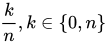For every positive , is a random variable with value Sample (Empirical) Distribution Function with Examples .

Since the unknown distribution Sample (Empirical) Distribution Function with Examples can be described, for example, by its distribution function , let us construct, from the sample, an «estimate» for this function.

Definition 1.

The empirical distribution function, constructed from the sample Sample (Empirical) Distribution Function with Examples of size , is the random function , which for each equals

$\begin{displaymath} F^*_n(y)=\dfrac{\textrm{ количество } X_i\in(-\infty,y)}{n} =\frac{1}{n}\sum\limits_{i=1}^n {\mathbf I}(X_i<y).\end{displaymath}$

Reminder: The random function

$\begin{displaymath} {\mathbf I}(X_i<y)=\begin{cases} 1, & \textrm{ если } X_i<y, \cr 0 & \textrm{ иначе } \end{cases}\end{displaymath}$

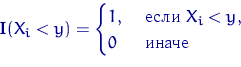
is called the indicator of the event Sample (Empirical) Distribution Function with Examples . For each this is a random variable having a Bernoulli distribution with parameter .

In other words, for any Sample (Empirical) Distribution Function with Examples the value , equal to the true probability that the random variable is less than , is estimated by the fraction of sample elements less than .

If the sample elements Sample (Empirical) Distribution Function with Examples , , are ordered in increasing order (for each elementary outcome), a new set of random variables is obtained, called the order statistics (variational series):

$\begin{displaymath} X_{(1)}\leqslant X_{(2)} \leqslant \ldots \leqslant X_{(n-1)}\leqslant X_{(n)}.\end{displaymath}$

Here

$\begin{displaymath} X_{(1)}=\min\{X_1, \ldots, X_n\}, \quad X_{(n)}=\max\{X_1, \ldots, X_n\}.\end{displaymath}$

The element Sample (Empirical) Distribution Function with Examples , , is called the -th term of the order statistics or the -th order statistic.

Main properties

Let an elementary outcome be fixed. Then is the distribution function of a discrete distribution given by the following probability function:

Sample (Empirical) Distribution Function with Examples ,

where Sample (Empirical) Distribution Function with Examples , and 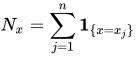is the number of sample elements equal to . In particular, if all sample elements are distinct, then .

The expected value of this distribution has the form:

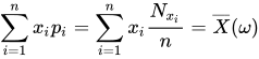Sample (Empirical) Distribution Function with Examples .

Thus, the sample mean is the theoretical mean of the sample distribution. Similarly, the sample variance is the theoretical variance of the sample distribution.

The random variable has a binomial distribution:

Sample (Empirical) Distribution Function with Examples .

The sample distribution function (x)} is an unbiased estimator of the distribution function :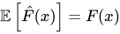

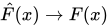Sample (Empirical) Distribution Function with Examples .

The variance of the sample distribution function has the form:

Sample (Empirical) Distribution Function with Examples .

By the strong law of large numbers, the sample distribution function converges almost surely to the theoretical distribution function:

Sample (Empirical) Distribution Function with Examples almost surely as .

The sample distribution function is an asymptotically normal estimator of the theoretical distribution function. If , then

Sample (Empirical) Distribution Function with Examples in distribution as .

Example 1.

Sample: ${\mathbf X}= (0;2;1;2{,}6;3{,}1;4{,}6;1;4{,}6;6;2{,}6;6;7;9;\ 9;2{,}6).$
Order statistics: $(0;1;1;2;2{,}6;2{,}6;2{,}6;3{,}1;4{,}6;4{,}6;6;\ 6;7;9;9).$

Sample (Empirical) Distribution Function with Examples

Fig. 1

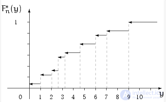
The empirical distribution function has jumps at the sample points; the size of the jump at the point Sample (Empirical) Distribution Function with Examples equals , where is the number of sample elements coinciding with .

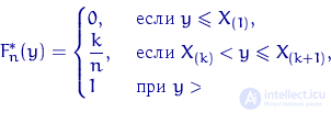
The empirical distribution function can be constructed from the order statistics as follows:

$\begin{displaymath} F_n^*(y)=\begin{cases} 0, & \textrm{ если } y\leqslant X_{(1... ...nt X_{(k+1)}, \cr 1 & \textrm{ при } y\gt X_{(n)}. \end{cases}\end{displaymath}$

Another characteristic of a distribution is the table (for discrete distributions) or the density (for absolutely continuous ones). The empirical, or sample, analog of the table or the density is the so-called histogram.

A histogram is constructed from grouped data. The presumed range of values of the random variable Sample (Empirical) Distribution Function with Examples (or the range of the sample data) is divided, independently of the sample, into a certain number of intervals (not necessarily equal). Let , , be intervals on the line, called the grouping intervals. For denote by the number of sample elements falling into the interval Sample (Empirical) Distribution Function with Examples :

$\begin{equation} \nu_j=\{\textrm{\,число } X_i \in A_j\}=\sum\limits_{i=1}^n {\m... ...A_j), \quad \textrm{ здесь } \quad \sum\limits_{j=1}^k \nu_j = n.\end{equation}$ (1)

Over each of the intervals Sample (Empirical) Distribution Function with Examples a rectangle is constructed, whose area is proportional to . The total area of all rectangles must equal one. Let be the length of the interval . The height of the rectangle over equals

$\begin{displaymath} f_j=\dfrac{\nu_j}{n l_j}.\end{displaymath}$

The resulting figure is called a histogram.

Example 2.

We have the order statistics (see Example 1):

$\begin{displaymath} (0;1;1;2;2{,}6;2{,}6;2{,}6;3{,}1;4{,}6;\ 4{,}6;6;6;7;9;9).\end{displaymath}$

Let us divide the segment Sample (Empirical) Distribution Function with Examples into 4 equal segments. Into the segment fell 4 sample elements, into — 6, into — 3, and into the segment 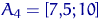fell 2 sample elements. We construct the histogram (Fig. 2). In Fig. 3 there is also a histogram for the same sample, but with the range divided into 5 equal segments.

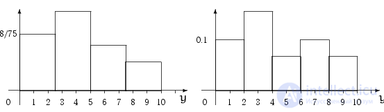
Sample (Empirical) Distribution Function with Examples

Fig. 2, Fig. 3

Remark 1.

In the course «Econometrics» it is asserted that the best number of grouping intervals («Sturges' formula») is Sample (Empirical) Distribution Function with Examples .

Here Sample (Empirical) Distribution Function with Examples is the decimal logarithm, so , i.e., when the sample size is doubled, the number of grouping intervals increases by 1. Note that the more grouping intervals there are, the better. But if one takes the number of intervals, say, of order , then as Sample (Empirical) Distribution Function with Examples grows the histogram will not approach the density.

The following statement holds:

If the density of the distribution of the sample elements is a continuous function, then as Sample (Empirical) Distribution Function with Examples in such a way that , pointwise convergence in probability of the histogram to the density takes place.

So the choice of the logarithm is reasonable, but it is not the only possible one.

Sample (Empirical) Distribution Function with Examples

Definition

Main properties

See also

See also

Comments

To leave a comment

Lectures and tutorial on "Probability theory. Mathematical Statistics and Stochastic Analysis"

Terms: Probability theory. Mathematical Statistics and Stochastic Analysis