
Lecture
Survival analysis (Rus. анализ выживаемости) — a class of statistical models that make it possible to estimate the probability of an event occurring.
Survival analysis is a branch of statistics devoted to the analysis of the expected duration of time until the occurrence of one event, such as death in biological organisms and failure in mechanical systems. This topic is called reliability theory, reliability analysis, or reliability engineering in engineering, duration analysis or duration modelling in economics, and event history analysis in sociology. Survival analysis attempts to answer certain questions, for example, what proportion of a population will survive past a certain time? Of those who survive, at what rate will they die or fail? Can multiple causes of death or failure be taken into account? How do certain circumstances or characteristics increase or decrease the probability of survival?
To answer these questions, it is necessary to define the notion of «lifetime». In the case of biological survival, death is unambiguous, but in the case of mechanical reliability, failure may not be well defined, since there can well exist mechanical systems in which failure is partial, gradual in nature, or not otherwise localised in time. Even in biological problems, some events (for example, a heart attack or the failure of another organ) may have the same ambiguity. The theory set out below assumes the existence of well-defined events at specific points in time; other cases may be better described by models that explicitly account for ambiguous events.
More generally, survival analysis involves the modelling of time-to-event data; in this context, death or failure is considered an «event» in the survival analysis literature – traditionally, only one event occurs for each subject, after which the organism or mechanism dies or fails. Models for recurring or multiple events relax this assumption. The study of recurring events is relevant to system reliability, as well as to many areas of the social sciences and medical research.
Survival analysis is concerned with modelling the processes by which terminal (critical) events occur for the elements of a given population (originally — «deaths» for the elements of a population of living beings). Thus, within medical research, survival analysis can answer such questions as «what proportion of patients will be surviving some time after the treatment techniques applied?», «what mortality rates will be observed among survivors?», «what factors affect the increase or decrease of the chances of survival?» and so on.
To answer the corresponding questions, it is necessary to be able to clearly define the «lifetime» of an element (the period during which the element remains in the population before the terminal event occurs). In the case of biological survival, «death» is unambiguous, but in other cases the occurrence of the terminal event cannot always be localised to a single point in time.
On the whole, survival analysis consists of building models that describe data on the time of occurrence of an event. Since a living organism can die only once, this approach traditionally considers only single, one-time terminal events.
Censoring is a form of the missing-data problem in which the time to an event is not tracked, for reasons such as the study ending before all enrolled participants have exhibited the event of interest, or a participant leaving the study before the event occurred. Censoring is frequently encountered in survival analysis.
If only a lower bound l is known for the true event time T, with T > l, this is called right censoring. Right censoring will occur, for example, for those subjects whose date of birth is known but who are still alive at the moment the data are lost to follow-up or the study ends. We usually encounter data censored by right censoring.
If the event of interest has already occurred before the subject was enrolled in the study, but it is not known when it occurred, the data are said to be subject to left censoring. [ 24 ] When it can only be said that the event occurred between two observations or examinations, this is interval censoring.
Left censoring occurs, for example, when a permanent tooth has already erupted before the start of a dental study whose goal is to estimate the distribution of its eruption. In the same study, eruption time is subject to interval censoring when the permanent tooth is present in the mouth at the current examination but was not yet present at the previous examination. Interval censoring is often encountered in HIV/AIDS research. Indeed, the time to HIV seroconversion can only be determined by a laboratory test, which is usually performed after a visit to the doctor. In such a case, one can only conclude that HIV seroconversion occurred between two examinations. The same is true for AIDS diagnosis, which is based on clinical symptoms and must be confirmed by a medical examination.
It may also happen that subjects with a lifespan below a certain threshold may not be observed at all: this is called truncation. Note that truncation differs from left censoring, since for left-censored data we know that the subject exists, but for truncated data we may have no knowledge of the subject whatsoever. Truncation is also common. In a so-called delayed-entry study, subjects are not observed at all until they reach a certain age. For example, people may not be observed until they reach school entry age. Any subjects who died in the pre-school age group will be unknown. Left-truncated data are common in actuarial work for life insurance and pensions.
Left-censored data can arise when a person's survival time becomes incomplete on the left side of their observation period. For example, in an epidemiological example, we may follow a patient for an infectious disease starting from the moment a positive test result for the infection is obtained. Although we may know the right-hand part of the duration of interest, we will never know the exact time of exposure to the infectious agent.
Data analysis using survival analysis methods can only be performed on censored data. Observations are called censored if the dependent variable of interest represents the moment of occurrence of the terminal event, and the duration of the study is limited in time.
With fixed censoring, a sample of n objects is observed over a fixed time. The number of objects for which the terminal event occurs, or the number of deaths, is random, but the total duration of the study is fixed. Each object has a maximum possible observation period i
 , i=1,…,n
 , which may vary from one object to another but is fixed in advance. The probability that object i will be alive at the end of its observation period is S(i)
 , and the total number of deaths is random.
With random censoring, a sample of n objects is observed for as long as necessary until d objects have experienced the event. In this scheme, the number of deaths d, which determines the precision of the study, is fixed in advance and can be used as a parameter. The drawback of this approach is that in this case the total duration of the study is random and cannot be known precisely in advance.
When censoring, one can specify the direction in which censoring is performed.
Right censoring occurs if the researcher knows at what point the experiment was started and that it will end at a point in time located to the right of the experiment's starting point.
If the researcher does not have information about when the experiment began (for example, in biomedical research it may be known when a patient was admitted to hospital and that they survived for a certain time, but information on when the symptoms of their disease first appeared may be missing), then left censoring is present.
Single censoring occurs at a single point in time (the experiment ends after some fixed time). On the other hand, in biomedical research multiple censoring naturally arises, for example, when patients are discharged from hospital after undergoing treatment of varying extents (or different durations), and the researcher knows only that the patient survived up to the corresponding censoring point.
These tables can be regarded as «expanded» frequency tables. The range of possible times of occurrence of critical events (deaths, failures, etc.) is divided into a number of time intervals (points in time). For each point in time, the number and proportion of objects that were part of the elements of the population under study (were «alive») at the start of the interval in question are calculated, as are the number and proportion of elements that left the population («died»), and the number and proportion of elements that were withdrawn or censored in each interval.
The object of analysis in the survival function is conventionally denoted as S; it is described by the following function:

where t — is some time during which the population was observed, T is a random variable denoting the moment of «death» (the object leaving the population), and
  denotes the probability of «death» in a given time interval. That is, the survival function describes the probability of «death» some time after moment t.
It is usually assumed that S(0)=1, although this value may be less than 1 if there is a possibility of immediate death or failure.
If u≥t, then the survival function must have the form S(u)≤S(t). This property follows from the fact that the condition T>u implies that T>t. Essentially, this implies that survival over a later period is only possible after surviving the earlier period.
It is usually assumed that the survival function tends to zero as the time variable increases without bound: S(t)→0 as t→∞ .
.
Survival analysis also uses the cumulative distribution function F(t) and its derivative — the probability density function f(t).
The cumulative distribution function has the form
F(t)=P(T≤t)=1−S(t)
and describes the probability that the terminal event has occurred by time t.
The probability density function (PDF) has the form
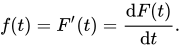
this function shows the frequency of occurrence of the terminal event at time t.
This is an estimate of the probability of leaving the population («death») in the corresponding interval, defined as follows:
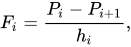
where Fi — is the estimate of the probability of failure in the i-th interval,  — is the cumulative proportion of surviving objects (the survival function) at the start of the i-th interval, i
 — is the width of the i-th interval.
The hazard function is defined as the probability that an element remaining in the population at the start of the corresponding interval will leave the population («die») during that interval. The estimate of the hazard-rate function is computed as follows:

The numerator of this expression is the conditional probability that the event will occur in the interval  , given that it has not occurred earlier, and the denominator is the width of the interval.
This is the point on the time axis at which the cumulative survival function equals 0.5. Other percentiles (for example, the 25th and 75th percentiles, or quartiles) of the cumulative survival function are calculated on the same principle.
Survival models can be meaningfully represented as linear regression models, since all of the distribution families listed above can be reduced to linear ones by means of suitable transformations. In this case, lifetime will be the dependent variable.
Knowing the parametric family of distributions, one can compute the likelihood function from the available data and find its maximum. Such estimates are called maximum-likelihood estimates. Under quite general assumptions, these estimates coincide with least-squares estimates. Similarly, the maximum of the likelihood function is found under the null hypothesis, that is, for a model that allows different rates in different intervals. The hypothesis formulated can be tested, for example, using the likelihood-ratio test, whose statistic has an asymptotic chi-squared distribution.
In general, a life table gives a good representation of the distribution of failures or deaths of objects over time. However, for forecasting it is often necessary to know the shape of the survival function under consideration.
Within survival analysis, the following families of distributions are most often used for building models:
For censored but ungrouped lifetime observations, the survival function can be estimated directly (without a life table). Suppose there exists a database in which each observation contains exactly one time interval. Multiplying the survival probabilities in each interval, we obtain the following formula for the survival function:
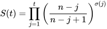
In this expression, S(t) — is the estimate of the survival function, n — is the total number of events (end times), j — is the (chronological) ordinal number of an individual event, σ(j) equals 1 if the j
 -th event denotes failure (death), and 0 if the j-th event denotes loss to follow-up (censoring); it denotes the product over all observations j completed by time t.
This estimate of the survival function, called the product-limit estimate, was first proposed by Kaplan and Meier (1958).
Survival analysis is used in several ways:
The following terms are commonly used in survival analysis:
The Cox-PH regression model is linear. It is analogous to linear and logistic regression. In particular, these methods assume that a single line, curve, plane, or surface is sufficient to separate groups (alive, dead) or to estimate a quantitative response (survival time).
In some cases, alternative partitions give more accurate classification or quantitative estimates. One alternative method is tree-based survival models, [ 12 ] [ 13 ] [ 14 ], including survival random forests. [ 15 ] Tree-based survival models can produce more accurate predictions than Cox models. A reasonable strategy is to consider both types of models for a given dataset.
This example of survival tree analysis uses the R package "rpart". [ 16 ] The example is based on data from 146 patients with stage C prostate cancer in the stagec dataset in rpart. Rpart and the stagec example are described in the work of Atkinson and Therneau (1997), [ 17 ], which is also distributed as a brief guide to the rpart package. [ 16 ]
Stage variables:
The survival tree resulting from the analysis is shown in the figure.
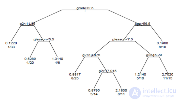
Survival tree for the prostate cancer dataset
Each branch of the tree indicates a split on the value of a variable. For example, the root of the tree splits subjects with a score < 2.5 and subjects with a score of 2.5 or higher. The terminal nodes indicate the number of subjects in the node, the number of subjects who experienced events, and the relative frequency of events compared to the root. In the leftmost node, the values 1/33 indicate that one of 33 subjects in the node experienced an event, and the relative frequency of events is 0.122. In the rightmost bottom node, the values 11/15 indicate that 11 of 15 subjects in the node experienced an event, and the relative frequency of events is 2.7.
An alternative to building a single survival tree is to build multiple survival trees, each built on a sample of the data, which are then averaged to predict survival. [ 15 ] This method underlies survival random forest models. Survival random forest analysis is available in the R package "randomForestSRC". [ 18 ]
The randomForestSRC package includes an example of survival random forest analysis using the pbc dataset. This data is taken from a study of primary biliary cirrhosis of the liver (PBC) conducted at the Mayo Clinic between 1974 and 1984. In this example, the survival random forest model gives more accurate survival predictions than the Cox PH model. Prediction errors are estimated using the bootstrap resampling method.
Recent advances in deep representation learning have been extended to survival estimation. The DeepSurv model [ 19 ] proposes to replace the log-linear parameterization of the CoxPH model with a multilayer perceptron. Further extensions such as Deep Survival Machines [ 20 ] and Deep Cox Mixtures [ 21 ], propose using latent-variable mixture models to model the distribution of time-to-event as a mixture of parametric or semi-parametric distributions while jointly learning representations of the input covariates. Deep learning methods have shown superior performance, especially on complex input data modalities such as images and clinical time series.
The object of primary interest is the survival function, conventionally denoted S, which is defined as S(t)=Pr(T>t) where t — is some point in time, T — is a random variable denoting the time of death or, more generally, any event, and «Pr» denotes probability. That is, the survival function is the probability of observing an event that occurred at a time later than a given time t. [ 7 ] The survival function is also called the survivor function or survivorship function in problems of biological survival and the reliability function in problems of mechanical survival. [ 22 ] In the latter case, the reliability function is denoted R(t).
It is usually assumed that S(0) = 1, although it may be less than 1 if there is a probability of immediate death or failure.
The survival function must be non-increasing: S(u) ≤ S(t), if u ≥ t. This property follows directly from the condition, since T > u implies T > t. This reflects the idea that surviving to a later age is only possible after reaching all younger ages. Given this property, the lifetime distribution function and the event density (F and f below) are well defined. [ 2 ]
It is usually assumed that the survival function tends to zero as age increases without bound (i.e. S(t) → 0 as t → ∞), although the limit may be greater than zero if eternal life is possible. For example, we could apply survival analysis to a mixture of stable and unstable carbon isotopes; the unstable isotopes will sooner or later decay, but the stable ones will exist indefinitely.
The corresponding quantities are defined in terms of the survival function.
The lifetime distribution function, conventionally denoted F, is defined as the complement of the survival function,
 If F is differentiable, then its derivative, which is the probability density function of lifetime, is usually denoted f.
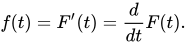 The function f is sometimes called the event density; it is the rate of occurrence of death or failure events per unit time.
The survival function can be expressed in terms of the probability distribution and probability density functions.
 Similarly, the survival event density function can be defined as
 In other fields, such as statistical physics, the survival event density function is known as the first passage time density.
The hazard function  is defined as the rate of events at timet,
 given survival up to timet.
Synonyms of the hazard function in various fields include the hazard rate, the intensity function, the force of mortality (demography and actuarial science, denotedμ ), the force of failure or failure rate (engineering, denoted
  ). For example, in actuarial science,
  denotes the mortality rate among people agedx
 , whereas in the field of engineering reliability
  denotes the failure rate of components after operating for a timet.
The hazard function represents the probability that a subject will experience the event in the next small interval of time, divided by the length of that interval, given that they have survived up to that point in time. . Formally, this can be written as follows:

where Bayes' theorem and the identification of  as the survival function were used in the first equality, and the definition of the lifetime probability density function — in the second.
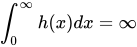
Any functionhis a hazard function if and only if it satisfies the following properties:
 ,
, .
.In fact, the hazard rate is usually more informative about the underlying failure mechanism than other representations of the lifetime distribution.
The hazard function must be non-negative,  , and its integral over[0,∞]
 must be infinite, but is otherwise unrestricted; it may be increasing or decreasing, non-monotonic, or discontinuous. An example is the «bathtub» hazard function, which is large for small values oft, decreasing to some minimum, and then increasing again; this can model the property of some mechanical systems to either fail shortly after being put into operation, or much later, as the system ages.
The hazard function can alternatively be represented as the cumulative hazard function, conventionally denotedΛ orH
orH :
:
 so, rearranging the signs and exponentiating
 or differentiating (with the chain rule)
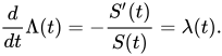 The name «cumulative hazard function» comes from the fact that
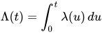 which represents the «accumulation» of hazard over time.
From the definition of  , we see that it increases without bound as t tends to infinity (assuming that
  tends to zero). This means thatλmust not decrease too quickly, since, by definition, the cumulative hazard must diverge. For example,
  is not the hazard function of any survival distribution, since its integral converges to 1.
The survival function ), the cumulative hazard function , the density  , the hazard function , and the lifetime distribution function
  are related through
Future lifetime at a given momentt0 is the time remaining until death, given survival to aget0. Thus, this isT−t0
 in the present notation. Expected future lifetime — is the expected value of future lifetime. The probability of death at or before reaching aget0+t
 , given survival to aget0, is simply
 Consequently, the probability density of future life is
 and the expected future lifetime is
 where the second expression is obtained by integration by parts.
For  , that is, at birth, this reduces to the life expectancy.
In reliability problems, expected lifetime is called the mean time to failure, and expected future lifetime is called the mean residual life.
Since the probability of an individual surviving to age t or longer is, by definition, equal to S(t), the expected number of survivors at age t from an initial population of n newborns is equal to n × S(t), assuming the same survival function for all individuals. Thus, the expected proportion of survivors is S(t). If the survival of different individuals is independent, the number of survivors at age t has a binomial distribution with parameters n and S(t), and the variance of the proportion of survivors is S(t) × (1 - S(t))/n.
The age at which a certain proportion of survivors will remain can be determined by solving the equation S(t) = q for t, where q — is the quantile of interest. Usually of interest is the median lifetime, for which q = 1/2, or other quantiles, for example, q = 0.90 or q = 0.99.

Comments