
Lecture
In spatial statistics, the theoretical variogram  is a function describing the degree of spatial dependence of a spatial random field or random process
  .
.
In the case of a specific example from the gold mining industry, the variogram gives a measure of how much two samples taken from the mining area will differ in gold content percentage depending on the distance between these samples. Samples taken far from each other will differ more than samples taken close to each other.
The variogram is a second-order statistical moment used in geostatistics for the analysis and modeling of spatial correlation.
The variogram  for values of the spatial variable
  at two points
  and
and  , separated by the vector
  , is defined by the variation (variance of the difference of the variable's values) at these points . Here the quantity
  is called the semivariogram:

If we accept the “intrinsic hypothesis”, that the increment of the function is weakly stationary, then the variance and mean of the increment  exist and do not depend on the location of the point


The variogram  was first defined by Matheron (Matheron, 1963) as half the average squared difference between points (
 and
and  ) separated by a distance of
  . Formally

where  is a point in the geometric field
  , and
, and  is the value at that point. For example, suppose we are interested in the iron content in soil samples in some region or field.. would be the content (e.g., in mg of iron per kg of soil) of iron at some location , where has latitude, longitude and elevation coordinates. The triple integral has more than three dimensions. represents the separation distance of interest (e.g. in m or km). To obtain the variogram for a given, all pairs of points at exactly that distance would be selected. In practice it is impossible to sample everywhere, so instead the empirical variogram is used.
The variogram is defined as
γ(si,sj) = ½ var(Z(si) - Z(sj)),
where var is the variance.
If two locations, si and sj, are close to each other in units of distance d(si, sj), one can expect them to be similar, so that the difference of their values, Z(si) – Z(sj), will be small. As i and sj move further apart from each other they become less similar, so the difference of their values, Z(si) – Z(sj), will become larger. This can be seen in the following figure, which shows what a typical variogram consists of.
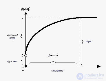
Note that the variance of the difference increases with distance, so the variogram can be regarded as a dissimilarity function. There are several terms that are often associated with this function, and they are also used in the ArcGIS Geostatistical Analyst Extension. The height that the variogram reaches when it levels off is called the sill. It often consists of two parts: a discontinuity at the origin, called the nugget effect, and the partial sill; together they make up the sill. The nugget effect can further be divided into measurement error and micro-scale variation. The nugget effect is simply the sum of the measurement error and the micro-scale variation, and since either of these components may be equal to zero, the nugget effect may consist entirely of the first or the second component. The distance at which the variogram levels off to the sill is called the range
The variogram is defined as the variance of the difference between the field values at two points ( and , note the change of notation from to  and
and  to
to  ) between realizations of the field (Cressie 1993):

or, in other words, this is twice the variogram. If the spatial random field has a constant mean value , this is equivalent to the expected square of the increment of values between locations and
  (Wackernagel 2003) (where and are points in space and possibly in time):

In the case of a stationary process, the variogram and the semivariogram can be represented as a function of the difference
  between locations only, by the following relation (Cressie 1993):

If the process is also isotropic, then the variogram and semivariogram can be represented by a function of the distance
 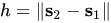 only (Cressie 1993):

The indices  or
or  are usually not written. These terms are used for all three forms of the function. Moreover, the term «variogram» is sometimes used to refer to the semivariogram, and the symbol
 is sometimes used for the variogram, which introduces some confusion.
According to (Cressie 1993, Chiles and Delfiner 1999, Wackernagel 2003), the theoretical variogram has the following properties:
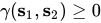 , since it is the expectation of a square.
 at distance 0 is always 0, since
  .
. subject to
  and locations
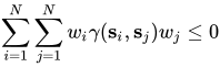
  it contains:
which corresponds to the fact that the variance
 of
of 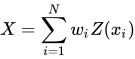 is given by the negation of this double sum and must be non-negative.
 For a non-stationary process it is necessary to add the square of the difference between the expected values at both points:
 if
if  ) the variogram is a constant
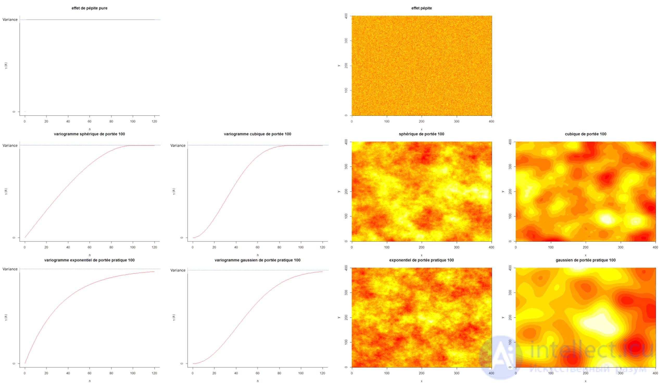
  everywhere except at the origin, where it is zero.
 is a symmetric function.
 is an even function.
 corresponds to the variance of the field. The bound of the variogram is also called its sill.
Generally, an empirical variogram is needed since sample information about is not available for all locations. Sample information might, for example, be the iron concentration in soil samples or pixel intensity on a camera. Each piece of sample information has coordinates for a 2D sample space, where and
  are geographic coordinates. In the case of iron in soil, the sample space may be three-dimensional. If there is also temporal variability (e.g., phosphorus content in a lake), then may be a four-dimensional vector
  . For the case where the dimensions have different units (e.g., distance and time), then a scaling factor
 may be applied to each to obtain a modified Euclidean distance.
Sample observations are denoted  . Samples can be taken at
  different locations in total. This will provide a set of samples
 at locations
  . Typically, graphs show the variogram values as a function of the separation of the sample points . For the empirical variogram, intervals of separation distances
 are used, rather than exact distances, and isotropic conditions are usually assumed (i.e. that is only a function of and does not depend on other variables, such as the central position). Then the empirical variogram
 can be calculated for each bin:

Or, in other words, each pair of points separated by (plus or minus some tolerance range of bin width  ) is found. They form a set of points
 . The number of these points in this bin is
 . Then for each pair of points
 , the square of the difference in the observation (e.g. soil sample content or pixel intensity) is found (
 ). These squared differences are summed and normalized by the number. By definition, the result is divided by 2 to obtain the variogram at that separation.
For computational speed, only unique pairs of points are needed. For example, for 2 pairs of observations [ ] taken from locations with separation only [] need to be considered, since the pairs [
 ] do not provide any additional information.
The empirical variogram is used in geostatistics as a first estimate of the (theoretical) variogram needed for spatial interpolation by kriging.
According to (Cressie 1993), for observations  from a stationary random field , the empirical variogram with lag tolerance 0 is an unbiased estimator of the theoretical variogram, due to:

The following parameters are often used to describe variograms:
 : The height of the jump of the variogram at the discontinuity at the origin.: The limit of the variogram as it tends to infinite lag distance.
 : The distance at which the difference between the variogram and the sill becomes negligible. In models with a fixed sill, this is the distance at which it is first reached; for models with an asymptotic sill, the convention is to use the distance when the semivariance first reaches 95% of the sill.
The empirical variogram cannot be calculated at every lag distance , and due to variation in the estimate, it is not guaranteed that it is a valid variogram as defined above. However, some geostatistical methods, such as kriging, require valid variograms. Thus, in applied geostatistics, empirical variograms are often approximated by a model function ensuring validity (Chiles & Delfiner 1999). Here are some important models (Chiles & Delfiner 1999, Cressie 1993):



The parameter  has different values in different references due to ambiguity in the definition of the range. For example
 is the value used in (Chiles & Delfiner 1999). In
 , the function equals 1 if
  and 0 otherwise.
In geostatistics, three functions are used to describe the spatial or temporal correlation of observations: these are the correlogram, the covariance, and the variogram. The latter is also more simply called the variogram. The sample variogram, unlike the variogram and semivariogram, shows where a significant degree of spatial dependence in the sample space, or where sample units scatter into randomness, when the point-of-view variance over time or per location of an ordered set is given as a function of the variance of the set and the lower bounds of its 99% and 95% confidence intervals.
The variogram is a key function of geostatistics, since it will be used to fit a model of the temporal/spatial correlation of the observed phenomenon. Thus, a distinction is made between the experimental variogram, which is a visualization of the possible spatial/temporal correlation, and the variogram model, which is further used to determine the weights of the kriging function. Note that the experimental variogram is an empirical estimate of the covariance in the form of a Gaussian process. Thus, it may not be positive definite and therefore cannot be used directly in kriging, without constraints and further processing. This explains why only a limited number of variogram models are used: most often these are the linear, spherical, Gaussian, and exponential models.
There is a relationship between the variogram and the covariance function.
γ(si, sj) = sill - C(si, sj),
This relationship can be seen in the figures. Because of this equivalence, interpolation can be performed in the ArcGIS Geostatistical Analyst Extension using either of these functions. (All variograms in the ArcGIS Geostatistical Analyst Extension have sills).
Variograms and covariances cannot be just any function. For interpolations to have non-negative kriging standard errors, only certain functions can be used as variograms and covariances. The ArcGIS Geostatistical Analyst Extension offers several acceptable options, and for the data one can try using different options. One can also have models constructed by adding several models together – such a construction provides valid models, and in the ArcGIS Geostatistical Analyst Extension up to four of them can be added. There are several cases where variograms exist but covariance functions do not. For example, there is a linear variogram, but it has no sill, and there is no corresponding covariance function. The ArcGIS Geostatistical Analyst Extension uses only models with sills. There are no reliable rules for choosing the "best" variogram model. By examining the empirical variogram or covariance function, the most suitable model can be chosen. Validation and cross-validation can also be used as a guide.
The covariance function is defined as
C(si, sj) = cov(Z(si), Z(sj)),
where cov is the covariance.
Covariance is a scaled version of correlation. If two locations, si and sj, are close to each other, one can expect them to be similar, and their covariance (correlation) will be large. As si and sj move further apart from each other they become less similar, and their covariance tends toward zero. This can be seen in the following figure, which shows what a typical covariance function consists of.
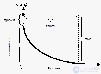
Note that the covariance function decreases with distance, so it can be regarded as a similarity function.
The square in the variogram, e.g.  , can be replaced with different powers: the madogram is defined with the absolute difference,
  , and the rodogram is defined by the square root of the absolute difference,
  . Estimators based on these lower powers are considered more robust to outliers. They can be generalized as a «variogram of order α»,
 ,
,
in which the variogram is of order 2, the madogram is a variogram of order 1, and the rodogram is a variogram of order 0.5.
When the variogram is used to describe the correlation of different variables, it is called a cross-variogram. Cross-variograms are used in co-kriging. If the variable is binary or represents classes of values, then it is referred to as an indicator variogram. The indicator variogram is used in indicator kriging.



Comments