
Lecture
One of the most important basic concepts of probability theory is the concept of a random variable.
A random variable (random quantity, random value) is a mathematical concept used to represent random phenomena for which a probability can be defined, that is, a measure of the possibility of occurrence.
Not to be confused with a random event.
The random variable is one of the basic concepts of probability theory. In mathematics, the Greek letter "xi"  is customarily used to denote a random variable.
A random variable is defined as follows. Let  be a probability space and
  a measurable space. Then a random variable on the sample space with values in the phase space is a
  measurable function
  .
.
Examples of objects whose states require the use of random variables are microscopic objects described by quantum mechanics. Random variables describe the transmission of hereditary traits from parent organisms to their offspring (see Mendel's laws). The radioactive decay of atomic nuclei is also a random event.
There are a number of problems in mathematical analysis and number theory for which the functions involved in their formulation are conveniently regarded as random variables defined on suitable probability spaces.
A random variable is a quantity that, as a result of an experiment, can take one value or another, and it is not known in advance which one.
Examples of random variables:
In all three examples above, the random variables can take separate, isolated values that can be listed in advance.
Thus, in example 1) these values are:
0, 1, 2, 3;
in example 2):
1, 2, 3, 4, …;
in example 3)
0; 0.1; 0.2; …; 1.0.
Such random variables, which take only values separated from one another that can be listed in advance, are called discontinuous or discrete random variables.
There are random variables of another type, for example:
The possible values of such random variables are not separated from one another; they continuously fill some interval, which sometimes has sharply defined boundaries, but more often – vague, blurred boundaries.
Such random variables, whose possible values continuously fill some interval, are called continuous random variables.
The concept of a random variable plays a very important role in probability theory. Whereas "classical" probability theory operated mainly with events, modern probability theory prefers, wherever possible, to operate with random variables.
Let us give examples of techniques typical of probability theory for passing from events to random variables.
An experiment is performed in which some event may or may not occur. Instead of the event one can consider a random variable
  that equals 1 if the event occurs, and equals 0 if the event does not occur. The random variable is obviously discrete; it has two possible values: 0 and 1. This random variable is called the indicator random variable of the event . In practice it is often more convenient to operate with indicator random variables instead of events. For example, if a series of experiments is performed, in each of which the event may occur, then the total number of occurrences of the event equals the sum of the indicator random variables of the event over all the experiments. In solving many practical problems, this technique proves very convenient.
On the other hand, it is very often convenient, in order to calculate the probability of an event, to associate this event with some continuous random variable (or a system of continuous variables).
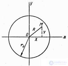
Fig. 2.4.1.
Suppose, for example, that the coordinates of some object O are measured in order to plot the point M representing this object on a panorama (layout) of the terrain. We are interested in the event that the error R in the position of the point M does not exceed a given value  (Fig. 2.4.1). Denote by
  the random errors in measuring the coordinates of the object. Obviously, the event is equivalent to the random point M with coordinates falling within a circle of radius centered at the point O. In other words, for the event to occur, the random variables and
  must satisfy the inequality
 . (2.4.1)
The probability of the event is nothing other than the probability that inequality (2.4.1) holds. This probability can be determined if the properties of the random variables are known.
Such an organic connection between events and random variables is very characteristic of modern probability theory, which, wherever possible, passes from the "scheme of events" to the "scheme of random variables". Compared with the former, the latter scheme is a much more flexible and universal apparatus for solving problems related to random phenomena.
The role of the random variable as one of the basic concepts of probability theory was first clearly recognized by P. L. Chebyshev, who substantiated the point of view on this concept that is generally accepted today (1867) . The understanding of a random variable as a special case of the general concept of a function came considerably later, in the first third of the 20th century. The first complete formalized presentation of the foundations of probability theory on the basis of measure theory was developed by A. N. Kolmogorov (1933) , after which it became clear that a random variable is a measurable function defined on a probability space. In the textbook literature, this point of view was first consistently carried through by W. Feller (see the preface to , where the exposition is built on the concept of a sample space and it is emphasized that only in this case does the notion of a random variable become meaningful).
The probability distribution of a random variable is the function  on the sigma-algebra
  of the phase space, defined as follows:
 , where
  (the probability distribution
  is a probability measure on the phase space ).
If the phase space of the random variable is the set of real numbers  with the Borel σ-algebra, then the distribution function
  equals the probability that the value of the random variable is less than the real number
  . It follows from this definition that the probability that the value of the random variable falls in the interval [a, b) equals
  . The advantage of using the distribution function is that it makes it possible to achieve a uniform mathematical description of discrete, continuous and mixed discrete-continuous random variables. Nevertheless, there exist different random variables that have the same distribution functions. For example, if the random variable takes the values +1 and −1 with equal probability 1/2, then the random variables and
  are described by one and the same distribution function F(x).
If a random variable is discrete, then a complete and unambiguous mathematical description of its distribution is given by specifying the probability function  of all possible values of this random variable. Examples of discrete random variables are variables having the binomial and Poisson distribution laws.
Random functions  and
and  in the phase space are called equivalent if, for any set , the events
  and
and  coincide with probability one:
 , where
  is the operation of symmetric difference of two sets.
For a separable phase space, equivalence means that the variables and  coincide with probability one, i.e.
  .
.
The joint probability distribution of random variables  on the sample space in the corresponding phase spaces
  is the function
  defined on sets
  as
as
 .
.
The probability distribution  , as a function on the semiring of sets of the form
  in the product of spaces
  , is a distribution function. Random variables
  are called independent if for any
 .
.
For any family of distributions  in the corresponding phase spaces
  ( the parameter
  belongs to an arbitrary set
  ) there exists a family of random variables
  on some sample space in the corresponding phase spaces
  with distribution , independent of one another (i.e. any random variables
  ,
,  , are independent).
Random variables are classified and named according to the type of their phase space. For example:
is called integer-valued if, depending on the random outcome, it takes one of the values  with the corresponding probabilities
  .
. is called a multidimensional random variable or an
  -dimensional random vector (with respect to the Borel
  -algebra on
  ). Equivalent to this is the following definition: a vector
  , whose elements are random variables, is called a multidimensional random variable or a random vector.
 is called an -dimensional complex random vector (also with respect to the corresponding Borel -algebra).-dimensional linear space
  constructed as the convex hull of more than
  points that are a realization of a random vector in the space is called a random convex polytope.
Let  be a measurable space and the set of values of the parameter . A function
  of the parameter
  , whose values are random variables
 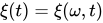 on the sample space in the phase space , is called a random process in the phase space . All possible joint probability distributions of the values
  :
:

are called the finite-dimensional probability distributions of the random process .
The mathematical expectation or mean value of a random variable in a normed linear space X on the sample space is the integral
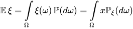
( assuming that the function is integrable).
The variance of a random variable is the quantity equal to:
 .
.
In statistics, the notation  or
or  is often used for the variance. The quantity , equal to

is called the root-mean-square deviation, the standard deviation, or the standard spread.
The covariance of random variables and is the following quantity:
 =
= 
(it is assumed that the mathematical expectation is defined).
If = 0, then the random variables and are called uncorrelated.
If  ,
, 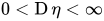 , then the quantity
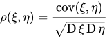
is called the correlation coefficient of the random variables.
The moment of order k of a random variable is the mathematical expectation  ; the absolute moment of order k is the quantity
  ; the central moment of order k is the quantity
  .
.
Let be an integer-valued random variable that, depending on the random outcome, takes one of the values with the corresponding probabilities . The function  of the variable
  ,
,  , defined by the formula
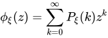 ,
,
is called the generating function of the distribution of the random variable . It is an analytic function of , , and the above formula gives its power series expansion. The probability distribution is uniquely determined by its generating function:

where  is the value of the derivative
  at the point z = 0.
The generating function for fixed coincides with the mathematical expectation of the random variable  :
:
 .
.
If the random variable has mathematical expectation  and variance
  , then
 ,
,
 .
.
For the generating function of a random variable equal to the sum  of independent random variables with generating functions
  , the following holds:
 .
.
Let  be a vector random variable in the -dimensional real space
  , where is the Borel -algebra. The function
  of the variable
  is called the distribution function of the random variable ( or the joint distribution function of the variables ). The function
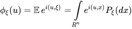 , where
  ,
,
of the variable  on the -dimensional real space is called the characteristic function of the random variable (or of the variables ). It is continuous and positive definite in the sense that
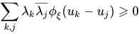
for any  and any numbers
  , and moreover
  . Every function
  possessing these properties is the characteristic function of some random variable .
Both the distribution function  and the characteristic function
  uniquely determine the probability distribution , , of the random variable .
If  , then in some neighborhood of the point
  the function
  (the branch of the logarithm equal to zero at zero) is continuously differentiable up to order
  . The value
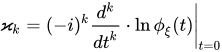
is called the cumulant of order k.
Let  be a sample space and some -algebra contained in
  . The conditional probability of an event
  with respect to the -algebra , denoted
  , is defined as a non-negative function of elementary outcomes
  ,
,  , measurable with respect to , for which
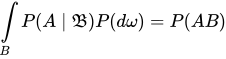
for any . The function on the set of elementary events  is uniquely defined for almost all elementary outcomes and is the density of the distribution
  , , with respect to the distribution
  on the -algebra
  .
.
The conditional probability  , considered as a function of with values in the normed space
  of all integrable (real and complex) functions on
 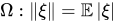 , is a generalized measure on the -algebra of the space , whose variation is
 .
.
Every random (real or complex) variable having a mathematical expectation (i.e. being an integrable function on the space with measure  ) is integrable with respect to the generalized measure . The corresponding integral
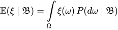
is called the conditional mathematical expectation of the random variable .
In terms of events, for a random variable and events  and
and  , provided that
 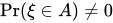 , Bayes' formula holds :

For a complete set of pairwise mutually exclusive events  and any event , taking into account the law of total probability :

Bayes' theorem holds:
 .
.
Different sources use different terminology for the various forms of Bayes' theorem.
If  is a Borel function and is a random variable, then its functional transformation
  is also a random variable. For example, if is a standard normal random variable, then the random variable
  has a chi-square distribution with one degree of freedom. Many distributions, including the Fisher distribution and the Student distribution, are distributions of functional transformations of normal random variables.
If and have the joint distribution  , and
, and  is some Borel function, then for
  the following holds :
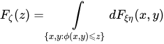 .
.
If  , and and are independent, then
  . Applying Fubini's theorem, we obtain:
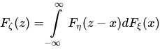
and similarly
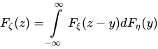 .
.
If  and
and  are distribution functions, then the function
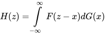
is called the convolution of and and is denoted  .
.
The characteristic function  of the sum of independent random variables and is the Fourier transform of the convolution of the distribution functions and and is equal to the product of the characteristic functions of and :
 .
.
Central limit theorems (CLTs) are a class of theorems stating that the sum of a large number of independent random variables with finite variances, each of which contributes only a small amount to the sum, has a distribution close to normal. The original source of research into the conditions under which the distribution of a sum of random variables converges to the normal distribution as their number increases was the local de Moivre–Laplace theorem.
A random variable can be specified, thereby describing all of its probabilistic properties as an individual random variable, by means of the distribution function, the probability density and the characteristic function, which determine the probabilities of its possible values.
Examples of a discrete random variable include speedometer readings or temperature measurements at specific moments in time.
All possible outcomes of a coin toss can be described by the sample space  heads, tails
 or, briefly,
  . Let the random variable equal the winnings from a coin toss. Suppose the winnings are 10 rubles each time the coin lands heads, and −33 rubles when it lands tails. Mathematically, this winnings function can be represented as follows:
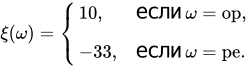
If the coin is fair, then the winnings will have a probability given by:
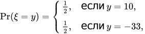
where  is the probability of winning
  rubles in a single coin toss.
A random variable can also be used to describe the process of rolling dice, as well as to calculate the probability of a particular outcome of such rolls. One classic example of this experiment uses two dice  and
and  , each of which can take values from the set {1, 2, 3, 4, 5, 6} (the number of pips on the faces of the dice). The total number of pips showing on the dice is the value of our random variable , which is given by the function:

and (if the dice are fair) the probability function for is given by:
 ,
,
where  is the sum of the pips on the dice that came up.
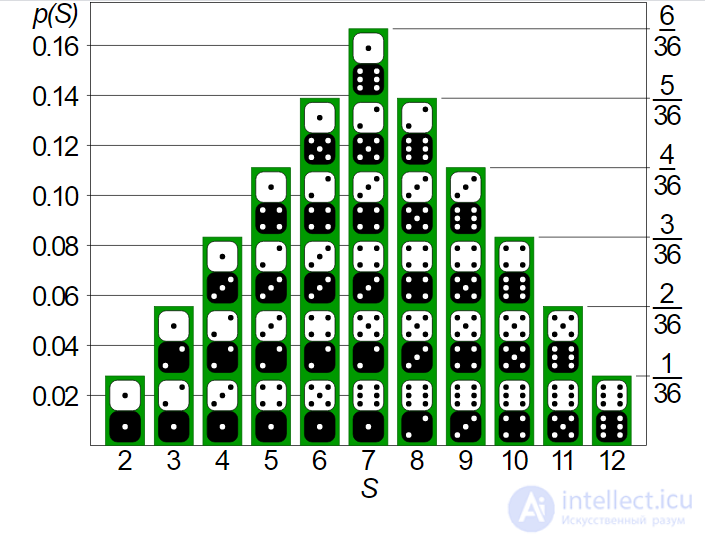
If the sample space is the set of all possible combinations of pips on two dice, and the random variable is equal to the sum of those pips, then S is a discrete random variable whose distribution is described by a probability function, the value of which is shown as the height of the corresponding column.
Suppose an experimenter draws one card at random from a deck of playing cards. Then will represent one of the drawn cards; here is not a number but a card, a physical object whose name is denoted by the symbol . Then the function  , taking the "name" of the object as its argument, will return a number that we will subsequently associate with the card . Suppose that in our case the experimenter drew the King of Clubs, that is,
  ; then, after substituting this outcome into the function
  , we obtain a number, for example, 13. This number is not the probability of drawing a king from the deck or any other card. This number is the result of translating an object from the physical world into an object of the mathematical world, since mathematical operations can now be performed with the number 13, whereas such operations could not be performed with the object
  .
.
The binomial distribution law describes random variables whose values determine the number of "successes" and "failures" when an experiment is repeated  times. In each trial, a "success" can occur with probability
  , and a "failure" with probability
  . In this case, the distribution law is determined by the Bernoulli formula:
 .
.
If, as tends to infinity, the product  remains equal to a constant
  , then the binomial distribution law converges to the Poisson law, which is described by the following formula:
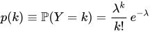 ,
,
where
 " denotes the factorial,
 is the base of the natural logarithm.
Another class of random variables consists of those for which there exists a non-negative function  satisfying, for any , the equality
 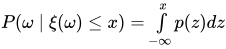 . Random variables satisfying this property are called continuous, and the function is called the probability density function.
The number of possible values of a continuous random variable is infinite. Examples of a continuous random variable: the measured speed of any type of vehicle, or the temperature over a specific time interval.
Suppose that in one experiment we need to select one person at random (denote them ) from a group of subjects, and let the random variable express the height of the person we selected. In this case, from a mathematical point of view, the random variable is interpreted as a function  that transforms each subject into a number, their height . To calculate the probability that a person's height falls between 180 cm and 190 cm, or the probability that their height is greater than 150 cm, we need to know the probability distribution of , which, together with , makes it possible to calculate the probabilities of various outcomes of random experiments.

Comments