Kinematics (Abstraction, Displacement, Velocity, Acceleration), Rotation of a Rigid Body, Projectile Motion at an Angle to the Horizontal

A typical problem of mechanics: knowing the state of a system (coordinates and velocities) at some initial moment of time , as well as the laws governing the motion, to determine the state of the system at all subsequent moments of time . For this purpose equations of motion are used — equations that make it possible to determine the position of a point particle (system) in space at any moment of time from known initial conditions. Experience shows that knowledge of the initial velocities and coordinates of the system is sufficient for tracing its subsequent fate. From a mathematical point of view, this means that the equations of motion do not contain time derivatives higher than the second (as it is said, these are second-order equations).

Why this is so — is a forbidden question. What these equations are — we shall see later on.

Kinematics operates with quantities such as displacement, distance travelled, velocity and acceleration.

2.1. Abstraction in Mechanics

No physical problem can be solved with absolute precision. Solving a problem approximately, one neglects certain factors that are not essential in the given case, that is, one abstracts from them. One of the abstractions in mechanics is the point particle (material point).

A mechanical system is a set of bodies singled out for consideration. If the linear dimensions of the bodies are small compared with the distances between them, and the rotation of the bodies about axes passing through them can be neglected, such a system may be regarded as consisting of point particles. For example, when calculating the travel time of a car, its linear dimensions can be neglected compared with the distance covered, that is, it can be treated as a point particle. But when studying the rotation of a car wheel, we must take into account its shape, mass and dimensions. In this case the first level of abstraction is no longer sufficient for us, and we move on to the next level.

The second level of abstraction includes the concept of an absolutely rigid body.

Here we do not neglect the dimensions of the body, but we assume the distances between any two of its points to be unchanging. At this level one can solve problems involving the rotation of wheels and pulleys, the operation of gyroscopes, and so on. In other words, those problems in which the deformations of the body are small compared with its linear dimensions.

But if we are interested precisely in the deformation of bodies, say, in calculations of bridges, the behaviour of beams and arches, then we leave the domain of classical mechanics and enter the domain of other scientific disciplines — theoretical mechanics, the theory of elasticity, and so on. In this course we shall confine ourselves to the first two levels of abstraction.

Since our space is three-dimensional, the number of degrees of freedom of a point particle equals three. For a system of point particles, between which there are no rigid constraints, the number of degrees of freedom naturally equals . When there are rigid constraints between the points, the number of degrees of freedom decreases by the number of such constraints. Thus, to uniquely specify the position of an absolutely rigid body in space we must give:

• three coordinates, fixing the position of some point of this body in space;

• two angles to determine the direction of an axis passing through the chosen point of the body;

• the angle of rotation of the body about this axis.

Note that the points of the body mentioned above need not necessarily lie on the surface of the absolutely rigid body or inside it; they must be rigidly connected to the body, that is, the distance from the chosen point to any point of the body must not change in the course of the motion.

Thus, the number of degrees of freedom of an absolutely rigid body is equal to six. For each degree of freedom of the system its own equation of motion must be written, that is, the number of scalar equations of motion of the system must coincide with the number of its degrees of freedom.

The fact that an absolutely rigid body has exactly six degrees of freedom can also be explained in the following way. It is fairly obvious that specifying the position of three points, rigidly connected to the body and not lying on one straight line, uniquely determines the position of the whole body in space. Such three points define a certain triangle. Three points have 9 degrees of freedom, but since these are points of an absolutely rigid body, the distances between them — the lengths of the sides of the triangle — are unchanging. These are three constraints, hence only six of the nine quantities remain independent: an absolutely rigid body has six degrees of freedom.

Specifying the three coordinates of some point rigidly connected to the body and the three angles determining the orientation of the body is convenient in that it suggests dividing all six degrees of freedom of the body into two kinds: three “translational” and three “rotational” degrees of freedom. We shall return to this question when considering the rotational motion of extended bodies.

2.2. Displacement

The concept of trajectory is essentially classical and loses its usual meaning in quantum mechanics. Depending on the shape of the trajectory, one distinguishes rectilinear motion, motion along a circle, and other kinds of curvilinear motion.

Note that besides the term “point particle (material point)” it is convenient to use the term “particle”, which is fully equivalent to it in this context. There is no need yet to associate it with elementary particles: protons, electrons, mesons and so on, of which there are many. That is, particle is simply another word for point particle.

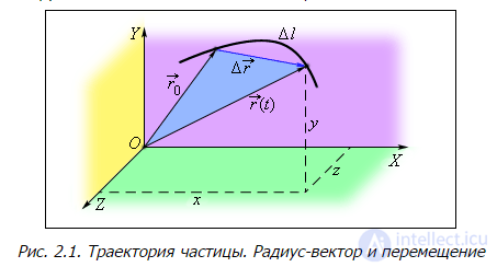
Fig. 2.1. Trajectory of a particle. Position vector and displacement

The position of the point particle in space is specified by the position vector (see Section 1.4). Since we are considering the motion of the point, the position vector depends on time:

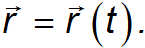
If at some moment of time t₁ the position of the point particle in space was r = r(t₁), and at moment of time t₂ it became r = r(t₂), then one speaks of the displacement of the point particle from point 1 to point 2 (Fig. 2.2.).

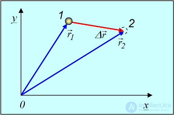
Fig. 2.2. Curvilinear motion of a particle

From Fig. 2.2. it is obvious that

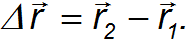
Displacement is a vector, characterized by the magnitude and direction, and displacements, as vectors should, add according to the parallelogram rule.

It is important to note that

Displacement must be distinguished from the distance travelled by the point particle.

Distance travelled is a non-negative, non-decreasing function of time. It may happen that the displacement is zero while the distance travelled reaches a considerable value. For example, in the morning you drive out of the garage, drive around town all day, and by evening park the car in the same spot. Since the initial and final positions coincide (), the displacement is zero:

while the distance travelled is recorded on the odometer.

To calculate the distance travelled, one must divide the trajectory into small segments (Fig. 2.3.).

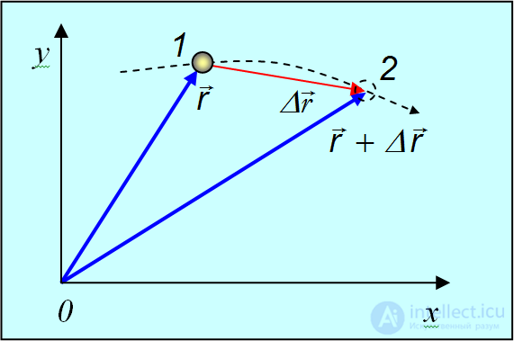
Fig. 2.3. Distance travelled and displacement for an infinitesimal displacement

Then the length of the displacement vector will be approximately equal to the distance travelled , and the coincidence will be the more exact the finer our subdivision. When subdivided into infinitesimal segments we have the equality

To find the total distance travelled we must sum all these infinitesimal distances, that is, compute the integral

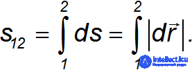
Here the integration is carried out along the trajectory from the initial point 1 to the final point 2.

The interactive model (Fig. 2.4.) illustrates the difference between distance travelled and displacement.

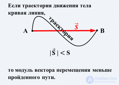
Fig. 2.4. Distance travelled and displacement

2.3. Velocity

Velocity — is a vector quantity characterizing not only how fast a particle moves along its trajectory, but also the direction in which the particle is moving at each moment of time.

The fact that this is precisely the average velocity we shall indicate by enclosing the averaged quantity in angle brackets: <...> , as done above.

The formula given above for the average velocity vector is a direct consequence of the general mathematical definition of the average value <f(x)> of an arbitrary function f(x) on the interval [a,b]:

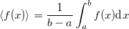
Indeed

The average velocity may turn out to be too crude a characteristic of motion. For example, the average velocity over a period of oscillation is always equal to zero, regardless of the nature of these oscillations, for the simple reason that over a period — by definition of the period — the oscillating body returns to its initial point and, consequently, the displacement over the period is always zero. For this and a number of other reasons, the instantaneous velocity is introduced — the velocity at a given moment of time. In what follows, when we mean the instantaneous velocity, we shall simply write “velocity”, omitting the words “instantaneous” or “at a given moment of time” whenever this cannot lead to misunderstanding.To obtain the velocity at moment of time t one must do the obvious thing: compute the limit of the ratio as the time interval t₂ – t₁ tends to zero. Let us make a change of notation: t₁ = t and t₂ = t + and rewrite the relation above in the form:

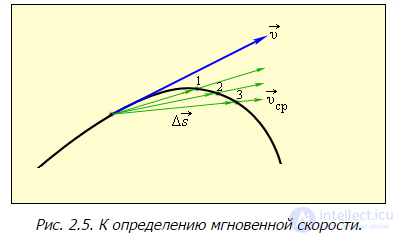
Fig. 2.5. On the definition of the instantaneous velocity.

At this point we are not considering the question of the existence of this limit, assuming that it exists. Note that if and are a finite displacement and a finite time interval, then and — are their limiting values: an infinitesimal displacement and an infinitesimal time interval. So the right-hand side of the definition of velocity

is nothing other than a fraction — the quotient of dividing by , so the last relation can be rewritten and is very often used in the form

Here and further on we shall often, for convenience, use the notation, going back to Newton, of the time derivative in the form of a dot over the corresponding quantity:

By the geometric meaning of the derivative, the velocity vector at each point of the trajectory is directed along the tangent to the trajectory at that point, in the direction of motion.

Video 2.1. The velocity vector is directed along the tangent to the trajectory. Experiment with a grinding wheel.

Any vector can be decomposed with respect to a basis (for the unit vectors of the basis, in other words, the unit vectors defining the positive directions of the axes OX,OY,OZ, we use the notations , , or , respectively). The coefficients of such a decomposition are the projections of the vector onto the corresponding axes. The following is important: in vector algebra it is proved that the decomposition with respect to a basis is unique. Let us decompose with respect to the basis the position vector of some moving point particle

Taking into account the constancy of the Cartesian unit vectors , , , let us differentiate this expression with respect to time

On the other hand, the decomposition of the velocity vector with respect to the basis has the form

comparing the two last expressions, taking into account the uniqueness of the decomposition of any vector with respect to a basis, gives the following result: the projections of the velocity vector on the Cartesian axes equal the time derivatives of the corresponding coordinates, that is

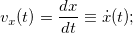
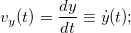
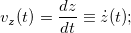
The magnitude of the velocity vector equals

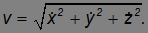
Let us obtain another, important, expression for the magnitude of the velocity vector.

It has already been noted that at the value || differs less and less from the corresponding distance travelled (see Fig. 2). Therefore

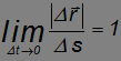
and in the limit (>0)

In other words, the magnitude of the velocity is the derivative of the distance travelled with respect to time.

Finally we have:

The average magnitude of the velocity vector, is defined as follows:

Here s(t₁, t₂) — is the distance travelled over the time from t₁ to t₂ and, correspondingly, s(t₀, t₂) — is the distance travelled over the time from t₀ to t₂ and s(t₀, t₂) — is the distance travelled over the time from t₀ to t₁.

The average velocity vector, or simply the average velocity, as indicated above, equals

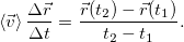
Note that, first of all, this is a vector; its magnitude — the magnitude of the average velocity vector — should not be confused with the average value of the magnitude of the velocity vector. In general they are not equal: the magnitude of the average vector is by no means equal to the average magnitude of this vector . The two operations, taking the magnitude and taking the average, cannot in general be interchanged.

Let us consider an example. Suppose a point moves in one direction. Fig. 2.6. shows a graph of the distance travelled s as a function of time (over the time from 0 to t). Using the physical meaning of velocity, find with the help of this graph the moment of time at which the instantaneous velocity equals the average path velocity over the first seconds of the point's motion.

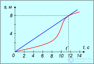
Fig. 2.6. Determination of the instantaneous and average velocity of a body

The magnitude of the velocity at the given moment of time

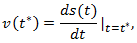
being the derivative of the distance with respect to time, equals the slope of the tangent to the graph of the dependence at the point corresponding to moment of time t*. The average magnitude of the velocity over the time interval from 0 to t* is the slope of the secant passing through the points of the same graph corresponding to the beginning t = 0 and the end t = t* of the time interval. We need to find the moment of time t* at which both slopes coincide. To do this, we draw through the origin of coordinates a straight line tangent to the trajectory. As can be seen from the figure, the point of tangency of this line with the graph s(t) gives t*. In our example we obtain

2.4. Calculation of the Distance Travelled and the Displacement

If the distance travelled by the point particle over the time interval from t₁ to t₂ is divided into sufficiently small segments , then for each -th segment the condition holds

Then the whole distance is approximately equal to the sum

As all the tend to zero, this approximate equality becomes exact, that is

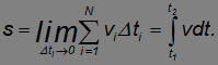
Let us stress that here we are talking about the magnitude of the velocity. If the dependence of the magnitude of the velocity on time is expressed graphically, then the distance travelled by the point particle over the time from t₂ to t₁ is numerically equal to the area of the figure bounded by the curve , the time axis, and the vertical lines passing through the points with abscissas and (Fig. 2.7.).

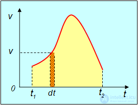
Fig. 2.7. Determination of the distance travelled from the graph of the dependence of velocity on time

In uniform motion, the value of the velocity is constant and can be taken outside the integral sign:

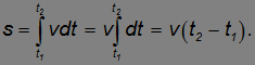
Since the magnitude of the velocity , the distance travelled by the body can only increase with time (or remain constant, when the body is at rest).

If we are interested in the displacement of the point particle over the same time, then we likewise divide the trajectory into small segments, but now we sum the vectors of displacement:

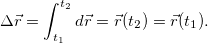
Taking into account the relation between displacement and the velocity vector

we obtain

In contrast to the expression for the distance travelled, here it is not the magnitude but the vector of velocity that stands under the integral. In just the same way, in uniform rectilinear motion, when , we can take the velocity outside the integral sign:

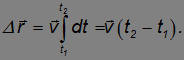
To actually find the displacement, the integral, presented in vector form, must be written in the form of integrals for the projections

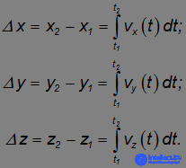
Here x₁, y₁, z₁ — are the coordinates of the point at moment of time t₁, and x₂, y₂, z₂ — are the coordinates of the point at moment of time t₂, respectively, and the magnitude of the displacement is then equal to

and the direction of the displacement vector is determined by the relation:

Example. Point A is located on a paved airfield, point B — on an adjoining field, on which the speed of the vehicle is n times less. In order to get from to in the shortest possible time, the optimal route shown in Fig. 2.8. was chosen. Find the relation between the sines of the angles α and β.

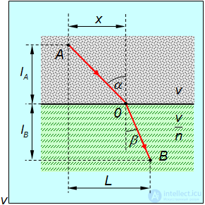
Fig. 2.8. Optimal route from point A to point B

All distances are shown in the figure. The time , spent on the path , covered at the speed , equals

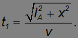
The time t₂, spent on the path , covered at the speed , equals

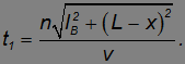
The total travel time will be

Since point 0 was chosen so that the minimum time was spent on the path, the derivative of the time with respect to the coordinate of the transition point from pavement to grass must equal zero:

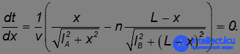
Since

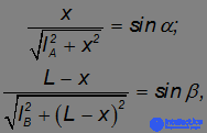
we find that

that is

The resemblance to the well-known law of refraction of light at the boundary between two media is no accident: nature is arranged so that light chooses the path requiring the minimum time. This is the so-called Fermat's principle, which we shall consider in detail in the corresponding section.

2.5. Acceleration of a Body

The velocity of a particle can change with time, both in magnitude and in direction.

The rate of change in time of any quantity is determined by the time derivative of that quantity. This general rule applies to the velocity vector as well.

Acceleration is equal to the derivative of the vector with respect to time t, or, equivalently, the second derivative with respect to time of the position vector :

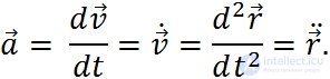
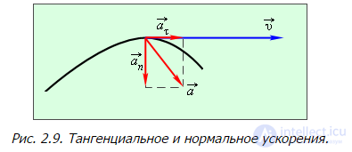
Fig. 2.9. Tangential and normal acceleration.

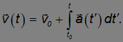
If the time dependence of the acceleration a = a(t) and the initial velocity v₀ (at t = t₀) are known, then the value of the velocity at any moment of time t is equal to

If the position of the body at the initial moment t = t₀ is also known, then we can find not only the velocity but also the position of the body at any moment of time:

In uniformly accelerated motion ( ) the integrals are easily computed and we obtain:

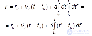
Evaluating the last integral leads to the law of uniformly accelerated motion of a point particle

In rectilinear motion the vectors of displacement, velocity and acceleration are directed along one and the same straight line, coinciding with the trajectory. Therefore the direction of the straight line can be taken as the x axis and one can operate with the acceleration and velocity as with projections of vectors onto this axis, that is, as algebraic quantities. In this case the index denoting the projection of a vector onto the axis is dropped.

Video 2.2. A cart rolling down an inclined plane as an example of uniformly accelerated motion.

2.6. Acceleration in curvilinear motion

Let us imagine a point particle moving along some curvilinear trajectory . Let us write the velocity in the form

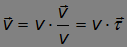
and note that the vector

— is the unit vector tangent to the trajectory and coinciding in direction with the velocity vector. Let us differentiate the velocity vector, written in this representation, and obtain

We have represented the acceleration in the form of two terms. Let us note first of all that the terms are orthogonal to each other. Indeed, since the vector — is a unit vector, then

Differentiating this scalar product, we obtain

that is

by the property of the scalar product.

Thus, we have decomposed the acceleration into the sum of two mutually orthogonal components, which we denote and :

Let us discuss the physical meaning of each term. The term

— is the tangential acceleration, which characterizes the rate of change of the magnitude of the velocity. This part of the total acceleration is directed either along the velocity, when the derivative dv/dt > 0, that is, the motion is accelerated, or opposite to the velocity, when this derivative dv/dt < 0, that is, the motion is decelerated. If the motion is uniform, dv/dt = 0, that is, the velocity, if it changes at all, changes only in direction, then the tangential part of the acceleration is equal to zero:

The term

is directed along the normal to the trajectory — perpendicular to the tangent to the trajectory — and is called the normal acceleration. If the tangential acceleration determines the rate at which the magnitude of the velocity vector changes, then the normal acceleration determines the rate at which the direction of the velocity vector changes.

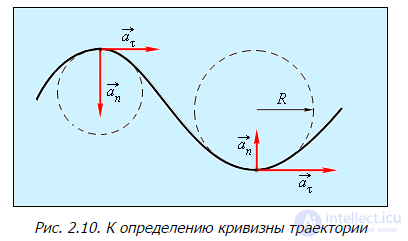
Fig. 2.10. On the definition of the curvature of the trajectory

Let us consider a “sufficiently smooth”, otherwise arbitrary, planar curvilinear trajectory. Planar, that is, all points of the trajectory lie in some plane — solely to simplify the derivation; the result obtained within this assumption is also valid for any “sufficiently smooth” spatial curve whose points cannot be fitted into a single plane. We will not consider the latter circumstance here; it is rigorously proved by the methods of analytic geometry. The words “sufficiently smooth” mean that the curve is described by a continuous function having continuous first and second derivatives. From the standpoint of physical applications, the requirement of the existence of continuous first two derivatives is in fact not a restriction on the shape of the trajectory, since it is practically always satisfied. Simply put, the trajectory must not have "corners" of the kind shown in figure 2.11.

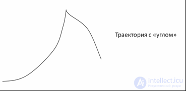
Fig. 2.11.

Such a “smooth” curve, on any of its infinitesimally small segments, can be replaced (fig. 2.12) by an arc of a circle of some radius. The radius of this circle, which approximates the trajectory on its infinitesimally small segment in the vicinity of some point, is customarily called the radius of curvature of the trajectory at that point. The centre of this circle is customarily called the centre of curvature of the trajectory at the given point. The curvature of the trajectory is the quantity C = 1/R. Let us emphasize that the radius of curvature, like the centre of curvature of the trajectory, is a local characteristic of it: each point of the trajectory has its own radius of curvature and its own centre of curvature. The exceptions are: 1) the circle, whose radius of curvature is the same at all its points and equal to the radius of the circle, the centre of curvature being “one for all” and coinciding with the centre of the circle, and 2) the straight line, for which at any point the radius of curvature is infinite, and the centre of curvature is located at a point infinitely far from the line. This is easy to understand: let us increase the radius of the circle — the larger the radius of the circle, the closer any of its finite segments is to a segment of a straight line. On a plain, best of all on a beach, from the height of a human being to the horizon is no more than five kilometres — within these limits the Earth is flat.

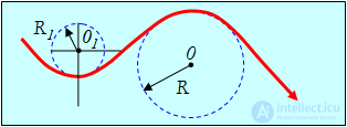
Fig. 2.12. On the definition of the radius of curvature of the trajectory

Let us compute the magnitude of the derivative entering the expression for the normal acceleration. The vector is directed along the normal to the trajectory toward the centre of curvature, as figure 2.13 makes clear.

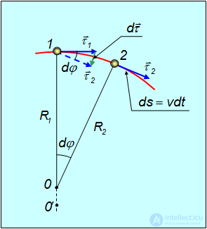
Fig. 2.13. Graphical determination of the radius of curvature of the trajectory

To do this, let us first go over from differentiation with respect to time to differentiation with respect to “path length”: , we have:

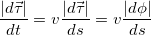
By definition, the derivative 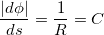is the curvature of the curve C, and the quantity inverse to it is equal to the radius of curvature of the curve R. Putting everything together, for the normal acceleration we finally obtain:

,

where the normal is perpendicular to the tangent and is always directed toward the centre of curvature, see fig. 11.

Let us give some additional explanation of figure 11. Take a point 2 close to point 1. Construct at these points the tangent unit vectors ₁ and ₂. The perpendiculars to these tangents will intersect at some point O₂. Note that for a curve which is not a circle, the distances R₁ and R₂ will differ slightly from each other. If we now move point 2 toward point 1, the intersection of the perpendiculars O₂ will move along the line O₂1 and in the limit will end up at some point O₁. The distances R₁ and R₂ will tend to a common limit R, equal to the radius of curvature, and the point O₁ will be the centre of curvature for point 1. Indeed, the circle of radius R centred at 0 passes through point 1 and is tangent to the trajectory (since the radius is orthogonal to the unit vector ₁). Moreover, by construction the infinitesimally close point 2 also lies on this circle. Thus, the constructed circle indeed “merges” with the trajectory at point 1.

Thus, in the general case the acceleration has two components — the tangential one

directed along the tangent and determining the rate of change of the magnitude of the velocity vector, and the normal one

directed perpendicular to the velocity toward the centre of curvature of the trajectory and proportional to the angular velocity of rotation of the velocity vector as the particle moves along the curvilinear trajectory (fig. 2.14).

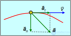
Fig. 2.14. Tangential and normal acceleration in accelerated curvilinear motion.

Indeed , where is precisely the angular velocity of rotation of the velocity vector .

The total acceleration

is determined by the parallelogram rule. The magnitude of the total acceleration, in accordance with the Pythagorean theorem, is equal to

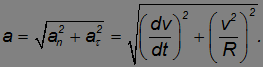
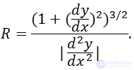
Let us write down, without derivation, the formulas relating the radius of curvature of a planar trajectory to the coordinates of the trajectory. If the dependence y = y(x) is known, then

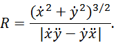
If, however, the trajectory is given in parametric form, x = x(t), y = y(t), then

An example of curvilinear motion with constant acceleration (a body thrown at an angle to the horizon) is shown in the following figure:

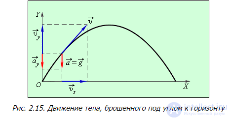
Fig. 2.15. Motion of a body thrown at an angle to the horizon

2.7. Motion of a body thrown at an angle to the horizon

Let us consider, as an example of the application of the formulas derived, the motion of a body thrown at an angle to the horizon in the absence of air resistance. Say, on a mountain, at a height above sea level, stands a cannon guarding coastal waters. Let a shell be fired at an angle to the horizon with initial velocity from a point , whose position is determined by the position vector (fig. 2.16).

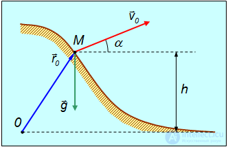
Fig. 2.16. Motion of a body thrown at an angle to the horizon

Supplement.

Derivation of the equations of motion of a point particle in a gravitational field

Let us write the equation of motion (the equation of Newton's second law):

As already noted, we take into account only the force of gravity .

The mass of the body cancels in the equation of motion

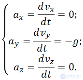
this means that bodies — point particles — of any masses, under the same initial conditions, will move in a uniform gravitational field identically. Let us project equation (2.7.2) onto the axes of a Cartesian coordinate system. The horizontal axis OX is shown in fig. 13 with a dotted line, the axis OY we draw through point O vertically upward, and the horizontal axis OZ, also passing through point O, we direct perpendicular to the vector toward us. We obtain:

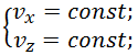
The vertical direction, by definition, is called the direction of the vector , hence its projections onto the horizontal axes OX and OY are equal to zero. In the second equation it is taken into account that the vector is directed downward, while the axis OY — upward.

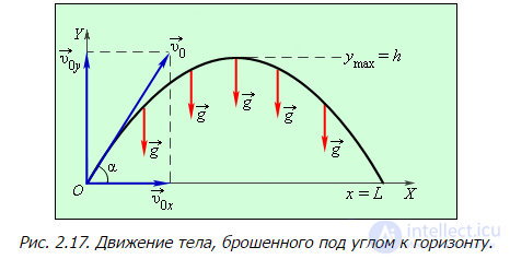
Fig. 2.17. Motion of a body thrown at an angle to the horizon.

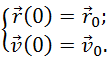
Let us add to the equations of motion the initial conditions, which determine the position and velocity of the body at the initial moment of time t₀, let t₀ = 0. Then, according to fig. 2.7.4

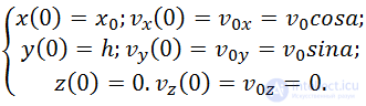
Or in projections onto the coordinate axes:

If the derivative of some function is equal to zero, then the function is constant; accordingly, from the first and third equations of (2.7.3) we obtain:

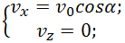
The constants are found from the initial conditions, namely: from the first and third equations of (2.7.5) it follows that at any moment of time

In the second equation of (2.7.3) the derivative is equal to a constant, whence it follows that the function depends linearly on its argument, that is

This constant is likewise found from the initial conditions. Substituting t = 0 into (2.7.8) and comparing the result (v_y(0) = const) with the second equation in (2.7.5) we obtain

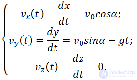
Combining (2.7.7) and (2.7.9), we obtain the final expressions for the dependences of the velocity projections on the coordinate axes on time:

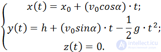
To determine the time dependences of the coordinates of the body, one more integration must be performed — integrate equations (2.7.10) with respect to time, taking into account the initial conditions (2.7.5). Using the same logic: if the derivative is equal to zero, then the function is constant; if the derivative is constant, then the function depends linearly on its argument; and choosing the constants so as to satisfy the initial conditions, one can obtain the following result:

The third equation of (2.7.11) shows that the trajectory of the body is planar, lying entirely in the plane XOY, this being a vertical plane defined by the vectors and . It is obvious that the latter statement is general: however the directions of the coordinate axes are chosen, the trajectory of a body thrown at an angle to the horizon is planar; it always lies in the plane defined by the vector of initial velocity and the vector of free-fall acceleration .

If we multiply the three equations of (2.7.10) by the unit vectors of the axes , , and and add them, and then do the same with the three equations of (2.7.11), we obtain the time dependences of the velocity vector of the particle and its position vector. Taking the initial conditions into account, we have:

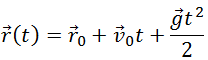
Formulas (2.7.12) and (2.7.13) could have been obtained at once, directly from (2.7.2), if one takes into account that the free-fall acceleration is a constant vector. If the acceleration — the derivative of the velocity vector — is constant, then the velocity vector depends on time linearly, while the position vector, whose time derivative is the linearly time-dependent velocity vector, depends on time quadratically. This is exactly what is recorded in relations (2.7.12) and (2.7.13), with constants — constant vectors — chosen in accordance with the initial conditions in the form (2.7.4).

From (2.7.13) it is in particular seen that the position vector is the sum of three vectors, added together according to the usual rules, which is clearly shown in fig. 2.18.

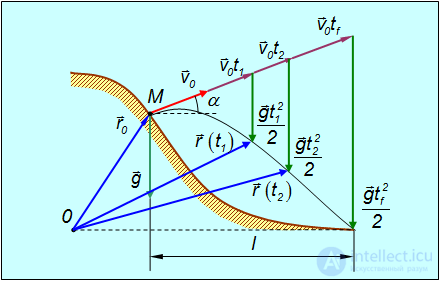
Fig. 2.18. Representation of the position vector r(t) at an arbitrary moment of time t as the sum of three vectors

These vectors represent:

• the initial position of the shell;

• the displacement (that is, as if there were no force of gravity);

• the displacement under the action of the force of gravity (free fall in the absence of initial velocity).

Here the principle of independence of motions is clearly manifested, known in other areas of physics as the principle of superposition. Generally speaking, according to the principle of superposition, the resulting effect of several influences is the sum of the effects of each influence taken separately. It is a consequence of the linearity of the equations of motion.

Video 2.3. Independence of horizontal and vertical displacements in motion in a gravitational field.

Let us place the origin at the point of throwing. Now =0, and let us orient the axes, as before, so that the axis 0x is horizontal, the axis 0y — vertical, and the initial velocity lies in the plane x0y (fig. 2.19).

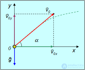
Fig. 2.19. Projections of the initial velocity onto the coordinate axes

Let us project onto the coordinate axes (see (2.7.11)):

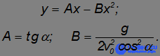
Trajectory of flight. If time t is eliminated from the resulting system of equations, we obtain the equation of the trajectory:

This is the equation of a parabola whose branches point downward.

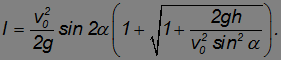
Range at a firing height h. At the moment the body lands, (the shell hits a target located at sea level). The horizontal distance from the cannon to the target is then equal to . Substituting ; into the equation of the trajectory, we obtain a quadratic equation for the range :

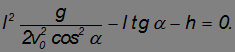
A quadratic equation has two solutions (in this case — a positive one and a negative one). We need the positive solution. The standard expression for the root of the quadratic equation of our problem can be brought to the form:

At this yields the well-known formula from the school physics course

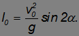
From it it follows, in particular, that the maximum range

is achieved at , if h = 0.

Maximum range. When firing from a mountain of height this is no longer the case. Let us find the angle at which the maximum range is achieved. The dependence of the range on the angle is rather complicated, and instead of differentiating to find the maximum we shall proceed as follows. Let us imagine that we increase the initial angle . At first the range increases (see formula (2.7.15)), reaches a maximum value and then begins to decrease again (to zero for a vertically upward shot). Thus, for every range except the maximum one, there correspond two directions of the initial velocity.

Let us return again to the quadratic equation for the range and consider it as an equation for the angle . Taking into account that

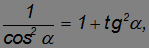
let us rewrite it in the form:

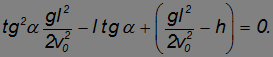
We have again obtained a quadratic equation, this time for the unknown quantity . The equation has two roots, corresponding to two angles at which the range is equal to . But when , both roots must coincide. This means that the discriminant of the quadratic equation is equal to zero:

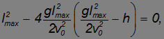
from which follows the result

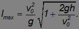
At this result reproduces formula (2.7.16)

Usually the height is much smaller than the range on level ground. At the square root can be approximated by the first terms of a Taylor series expansion, and we obtain the approximate expression

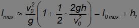
that is, the range of the shot increases by approximately the height by which the cannon is raised.

When l = l_max, and a = a_max, as already noted, the discriminant of the quadratic equation equals zero, and correspondingly its solution takes the form:

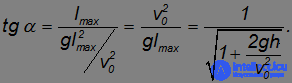
Since the tangent is less than unity, the angle at which the maximum range is achieved is less than .

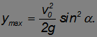
Maximum height of ascent above the initial point. This quantity can be determined from the vertical component of velocity being equal to zero at the top point of the trajectory

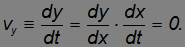
Here the horizontal component of velocity is not equal to zero, therefore

Differentiating the trajectory equation obtained earlier, we arrive at the equation:

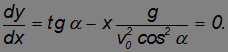
Hence

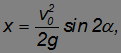
which, on substitution into the trajectory equation of the flight, leads to the formula:

Duration of flight. Since the horizontal component of velocity does not change, the duration of the flight is determined as the ratio of the range to the horizontal component of the initial velocity, that is

At we obtain

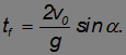
At (the gun fires in the horizontal direction) the flight time

is equal to the time of fall of a body from height . The range in this case

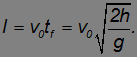
Distance travelled by the body. Over time t the body travels a distance

The integral can be taken in elementary functions, but because of the cumbersomeness of the answer we do not write out the corresponding expression here.

Distance from the point of firing. At time t the distance from the point of firing is determined by the magnitude of the position vector:

Radius of curvature of the trajectory at a given point. In the absence of air resistance the body moves with a constant acceleration due to gravity , which is also the total acceleration.

The tangential component of acceleration, characterizing the rate of change of the magnitude of the velocity, is equal to

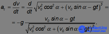
The normal component of acceleration, which changes the direction of the body's velocity, is determined by the relation:

Using the relation between the normal component of acceleration and the radius of curvature, we find :

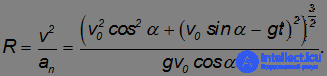
In the numerator of this expression the magnitude of the velocity appears raised to the power 3/2. Therefore, without even computing the derivative, we can answer the question of at which point of the trajectory the curvature is maximal, and the radius of curvature C = 1/R is minimal. The radius of curvature R reaches a minimum where the velocity is minimal, and this occurs at the top point of the trajectory, where the vertical component of velocity is equal to zero:

Let us recall once again that the horizontal component of velocity has the same value everywhere. At the top point the magnitude of velocity equals the horizontal component of velocity

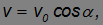
therefore

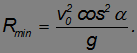
For comparison: the radius of curvature at the initial moment equals

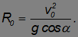
Position of the centre of curvature (for the highest point of the trajectory). By definition of the radius of curvature, the centre of curvature for the highest point of the trajectory lies directly below this point at a height

Let us recall that we measure vertical distances from the level of the gun, not from sea level.

At

this coordinate is negative, that is, the centre of curvature lies below the gun. The centre of curvature occupies its highest position at :

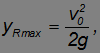
which coincides with the top point of the trajectory. Then the radius of curvature is equal to zero. This means that the curvature at this point is infinite, which is easy to verify by picturing the trajectory of vertical motion of a projectile.

2.8. Rotation of an absolutely rigid body

Let us consider the kinematics of motion of an extended body, whose dimensions cannot be neglected under the conditions of the problem at hand. We shall regard the body as non-deformable, in other words — absolutely rigid.

By a straight line “rigidly connected with the body” is meant a straight line the distance from any point of which to any point of the body remains constant during its motion.

Translational motion of an absolutely rigid body can be characterized by the motion of any single point of this body, since in translational motion all points of the body move with the same velocities and accelerations, and their trajectories are congruent. Having determined the motion of any one point of the rigid body, we thereby determine the motion of all its other points. Therefore describing translational motion raises no new problems compared with the kinematics of a point particle. An example of translational motion is shown in Fig. 2.20.

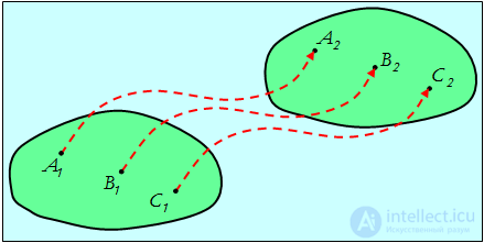
Fig.2.20. Translational motion of a body

An example of translational motion is shown in the following figure:

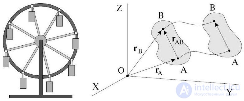
Fig.2.21. Plane motion of a body

Another important special case of the motion of a rigid body — is motion in which two points of the body remain fixed.

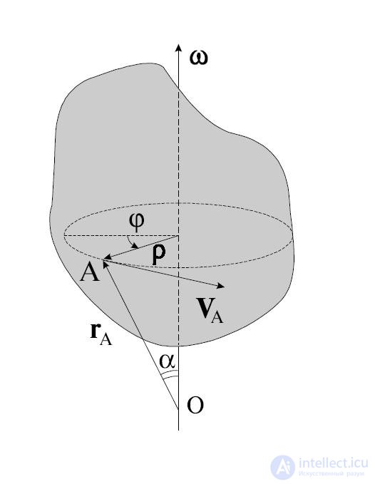
Fig.2.22. Rotation of a rigid body

In such motion all points of the body move along circles lying in planes perpendicular to the axis of rotation. The centres of the circles lie on the axis of rotation. In this case the axis of rotation can lie outside the body as well.

Video 2.4. Translational and rotational motion.

Angular velocity, angular acceleration. When a body rotates about some axis, all its points describe circles of different radii and, consequently, have different displacements, velocities and accelerations. Nevertheless, the rotational motion of all points of the body can be described in the same way. For this, kinematic characteristics of motion different from those of a point particle are used — the angle of rotation , the angular velocity , the angular acceleration .

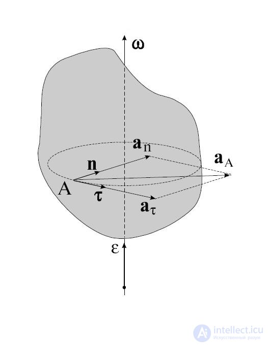
Fig. 2.23. Acceleration vectors of a point moving along a circle

The role of displacement in rotational motion is played by the vector of small rotation , about the axis of rotation 00' (Fig. 2.24.). It will be the same for any point of an absolutely rigid body (for example, points 1, 2, 3).

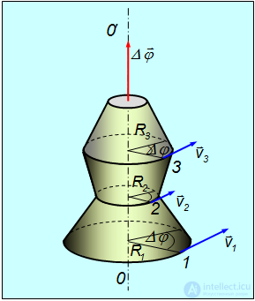
Fig. 2.24. Rotation of an absolutely rigid body about a fixed axis

The magnitude of the rotation vector equals the value of the angle of rotation , where the angle is measured in radians.

The vector of an infinitesimally small rotation is directed along the axis of rotation in the direction of motion of a right-hand screw (gimlet) turned in the same direction as the body.

Video 2.5. Finite angular displacements are not vectors, since they do not add by the parallelogram rule. Infinitesimally small angular displacements – are vectors.

Vectors whose directions are linked to the right-hand screw rule are called axial (from the English axis — axis) as opposed to polar vectors, which we have used previously. Polar vectors include, for example, the position vector, the velocity vector, the acceleration vector and the force vector. Axial vectors are also called pseudovectors, since they differ from true (polar) vectors in their behaviour under the operation of mirror reflection (inversion, or, equivalently, the transition from a right-handed to a left-handed coordinate system). It can be shown (this will be done later) that the addition of vectors of infinitesimally small rotations occurs in the same way as the addition of true vectors, that is, by the parallelogram (triangle) rule. Therefore, if the operation of mirror reflection is not considered, the difference between pseudovectors and true vectors does not manifest itself in any way, and they can and should be treated as ordinary (true) vectors.

The basic unit of measurement for the magnitude of angular velocity is rad/s. In printed publications, for reasons having no relation whatsoever to physics, one often sees 1/s or s^-1 written instead, which, strictly speaking, is incorrect. Angle is a dimensionless quantity, but its units of measurement vary (degrees, points of the compass, gradians …) and they must be specified, if only to avoid misunderstandings.

Video 2.6. The stroboscopic effect and its use for remote measurement of angular velocity of rotation.

The angular velocity , like the vector to which it is proportional, is an axial vector. When rotating about a fixed axis the angular velocity does not change its direction. In uniform rotation its magnitude also remains constant, so that the vector . In the case of sufficient constancy of the magnitude of angular velocity over time, it is convenient to characterize the rotation by its period T:

The words “sufficient constancy” mean, obviously, that over a period (the time of one revolution) the magnitude of the angular velocity changes insignificantly.

Also often used is the number of revolutions per unit time

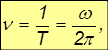
from which

In this case, in technical applications (above all, engines of all kinds) it is generally accepted to take not the second but the minute as the unit of time. That is, the angular velocity of rotation is given in revolutions per minute. As is easy to see, the relation between (in radians per second) and (in revolutions per minute) is as follows

The direction of the angular velocity vector is shown in Fig. 2.25.

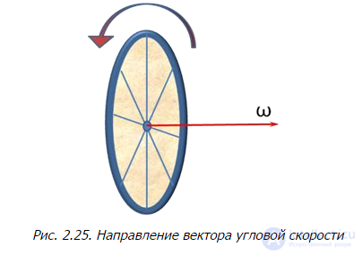
Fig. 2.25. Direction of the angular velocity vector

By analogy with linear acceleration, angular acceleration is introduced as the rate of change of the angular velocity vector. Angular acceleration is also an axial vector (pseudovector).

When rotating about a fixed axis, or, more generally, when rotating about an axis that remains parallel to itself, the angular velocity vector is likewise directed parallel to the axis of rotation. As the magnitude of the angular velocity || increases, the angular acceleration coincides with it in direction; as it decreases — it is directed the opposite way. Let us emphasize that this is only a special case in which the direction of the axis of rotation does not change; in the general case (rotation about a point) the axis of rotation itself turns, and then the above statement is not true.

Relation between angular and linear velocities and accelerations. Each point of a rotating body moves with a certain linear velocity , directed along the tangent to the corresponding circle (see Fig. 19). Let a point particle rotate about the axis 00' along a circle of radius R. In a small interval of time it will travel a distance , corresponding to an angle of rotation . Then

Passing to the limit , we obtain the expression for the magnitude of the linear velocity of a point on a rotating body.

Let us recall that here R — is the distance from the point of the body in question to the axis of rotation.

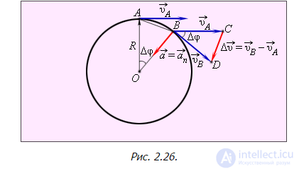
Fig. 2.26.

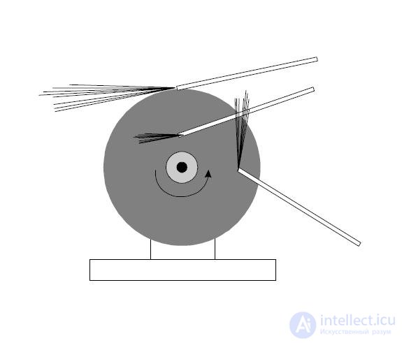
Fig. 2.27. Direction of the motion of sparks when grinding tools.

Since the normal acceleration is equal to

then, taking into account the relation between angular and linear velocity, we obtain

The normal acceleration of points of a rotating rigid body is often called centripetal acceleration.

Differentiating with respect to time the expression for , we find

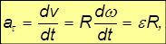
where — is the tangential acceleration of a point moving along a circle of radius R.

Thus, both the tangential and the normal accelerations grow linearly with increasing radius R — the distance from the axis of rotation. The total acceleration also depends linearly on R:

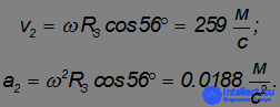
Example. Let us find the linear velocity and the centripetal acceleration of points lying on the Earth's surface at the equator and at the latitude of Moscow ( = 56°). We know the period of rotation of the Earth about its own axis T = 24 hours = 24x60x60 = 86 400 s. From this we find the angular velocity of rotation

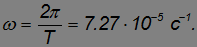
The mean radius of the Earth

The distance to the axis of rotation at latitude is equal to

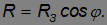
From this we find the linear velocity

and the centripetal acceleration

At the equator = 0, cos = 1, hence,

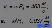
At the latitude of Moscow cos = cos 56° = 0.559 and we obtain:

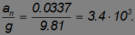
We see that the effect of the Earth's rotation is not so great: the ratio of the centripetal acceleration at the equator to the acceleration of free fall is equal to

Nevertheless, as we shall see later, the effects of the Earth's rotation are quite observable.

Relation between the vectors of linear and angular velocity. The relations obtained above between angular and linear velocity are written for the magnitudes of the vectors and . To write these relations in vector form, we use the notion of the vector (cross) product.

Let 0z — be the axis of rotation of an absolutely rigid body (Fig. 2.28).

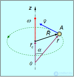
Fig. 2.28. Relation between the vectors of linear and angular velocity

Point A rotates along a circle of radius R. R — is the distance from the axis of rotation to the point of the body in question. Let us take point 0 as the origin of coordinates. Then

and since

then, by the definition of the vector product, for all points of the body

Here — is the position vector of the point of the body, starting at point O, lying at an arbitrary fixed location, necessarily on the axis of rotation

But, on the other hand

and

The first term is equal to zero, since the vector product of collinear vectors is equal to zero. Consequently,

where the vector R is perpendicular to the axis of rotation and directed away from it, and its magnitude is equal to the radius of the circle along which the point particle moves, and this vector begins at the centre of this circle.

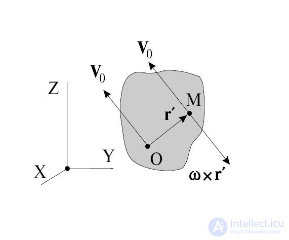
Fig. 2.29. On the definition of the instantaneous axis of rotation

The normal (centripetal) acceleration can also be written in vector form:

where the “–” sign shows that it is directed towards the axis of rotation. Differentiating the relation for linear and angular velocity with respect to time, we find for the total acceleration the expression

The first term is directed along the tangent to the trajectory of the point on the rotating body and its magnitude is equal to , since

Comparing with the expression for tangential acceleration, we arrive at the conclusion that this — is the vector of tangential acceleration

Consequently, the second term represents the normal acceleration of this same point:

Indeed, it is directed along the radius R towards the axis of rotation and its magnitude is equal to

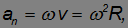
since

Therefore this relation for the normal acceleration is another form of writing the formula obtained earlier.