
Lecture
The subject of natural science in the broad sense is the understanding of the world around us. The task of the natural sciences is to form in our minds a model of the physical world that reflects its properties as fully as possible and provides relationships between the elements of the model that exist between the elements of the external world. J. Maxwell wrote “The exact sciences strive to reduce the riddles of nature to the determination of certain quantities by operations upon numbers”. Therefore the natural sciences “speak” to nature in the language of mathematics. The principle “nulla scientia potest sciri sine mathematika” (no science can be known without mathematics) was formulated as far back as the Middle Ages. But where do we get these very numbers that mathematics operates with, that must appear in the equations expressing this or that regularity of nature? The only source of them can be nature itself (we do not consider variants of “divine” revelation, as they are of little practical use).
I keep six honest serving-men,
(They taught me all I knew);
Their names are What and Why and When
And How and Where and Who.
R. Kipling
Natural science — is a complex of experimental sciences, at the foundation of which lie the most general regularities, studied by physics.
The natural sciences begin with observations and measurements, and are verified and nourished in their development by them. Of course, new ideas in science also arise thanks to speculative reasoning. But the final answer to the decisive questions can only be obtained through experiment. And these very ideas themselves do not arise out of nowhere.
With the help of instruments we pose questions to nature, and receive answers, which we “process” in our brain, on our computers. To understand a phenomenon means to be able to describe it, to know the conditions under which it occurs, to predict its consequences. It is important only to formulate our questions correctly, and then we get a chance that nature will answer them.
Nature (and science along with it) does not answer the question “why?”. Why does a body acquire acceleration under the action of a force? Why does an electric field act on a charge? Is anyone actually able to answer these questions? We can only state facts of the following type:
In other words, science in principle can answer only the question “how?”. How is our world arranged, what laws govern it, what is the mechanism of this or that process, what are their characteristic times and scales, by what equations are they described.
Physics studies the most fundamental regularities of nature, its simplest constituent parts. Thanks to this “simplicity” physics (just like chemistry, molecular biology, etc.) deals with reproducible situations. This means that we can repeat our experiments, and if all the conditions are satisfied exactly, the results will be the same. This is hardly possible, for example, in geology, not to mention the social sciences (economics, history, etc.). It is also important to understand that a physical experiment is never ideal, any measurement is carried out with a certain precision. And when we speak of this or that law of nature, we must remember that this law was established under certain specific conditions and, as a rule, has specific limits of applicability.
Physical models and theories are intended to bring into correspondence with one another the information that we obtain by studying natural phenomena. Not one of the theories can claim the title of being true, it only gives the best description, for the given time, of the domain in which it is applied. We call a theory “good” if it:
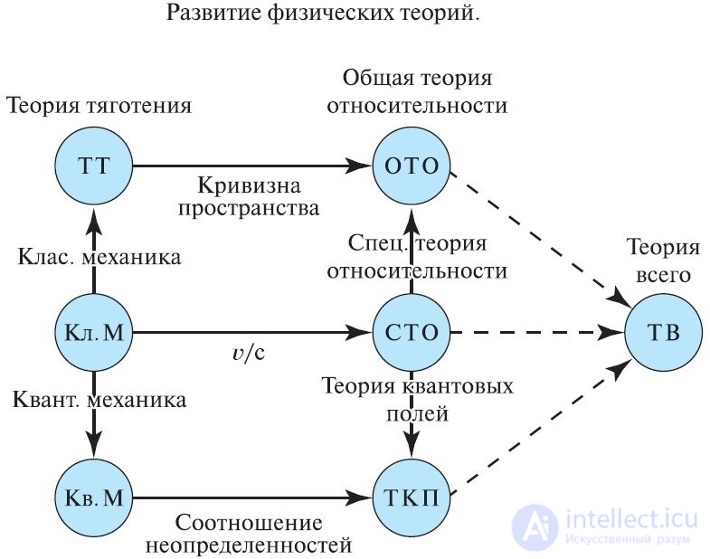
Fig. 1.1. Development of physical theories
The history of science has shown that, as a rule, a “good” theory allows for the possibility of improvement. This does not mean that a “good” theory is unconditionally true. A theory can always be changed (or completely rejected) if new facts become known. It is simply that with a deeper penetration into the essence of things, it turns out that a “good” theory is part of a more general theory and has its own domain of applicability. This is what happened, say, to Newtonian mechanics after the discovery of the theory of relativity.
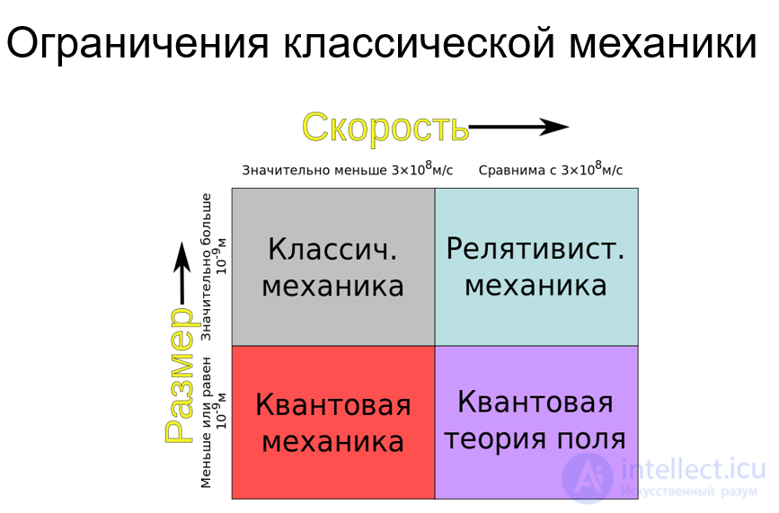
Limitations of classical mechanics
The results of numerous experimental observations are generalized in the form of physical laws, which represent certain statements concerning relations between one or another physical quantity. To test these statements experimentally it is necessary to measure by independent methods all the quantities that are related in a given physical law. The measurement of any physical quantity is carried out by comparing it with a certain standard value, taken as the unit of that quantity. These units must necessarily be indicated together with the numerical value of the result. The metric system of measures, created in the era of the Great French Revolution, was intended by its authors to serve “for all times, for all peoples, for all countries”.
Base units of measurement are chosen arbitrarily.
Let us clarify the fact that the choice of base units is arbitrary with the following examples. Length can be measured equally well in arshins, sazhens, feet, yards, metres and so on. The distance from Moscow to St. Petersburg by railway is 650 kilometres (km), this same distance in nautical miles (1 international nautical mile equals 1852 metres) is approximately 351 nautical miles. Mass can be measured in kilograms or, for example, in pounds. We may note: the British avoirdupois pound — 453.592 grams (g), the troy or apothecary pound — 373.242 g, the Russian pound (funt), used before the introduction of the metric system — 409.512 g.
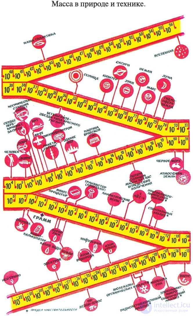
Fig. 1.2. Mass in nature and technology
For those who closely follow international gold trading, let us note that at these trades, by tradition, the price of a troy ounce of gold is quoted, that is, 31.1034768 grams (1/12 of an apothecary pound).
The purpose of the examples given is to show that the freedom (arbitrariness) of choosing base units of measurement can lead to quite costly confusion. In reality, the freedom to choose base units that claim, as stated above, to serve “for all times, for all peoples, for all countries”, is limited by a whole series of strict requirements. Namely (we quote from the book by A.G. Chertov, "The International System of Units of Measurement", Moscow, Rosvuzizdat, 1963):
1."The number of base units of the system must be reduced to a reasonable minimum. As the number of base units of the system increases, the number of dimensional coefficients in physical formulas also increases, which creates inconvenience when using the system.
Conversely, in a system with a smaller number of base units, the number of dimensional coefficients decreases. However, as the number of base units of the system decreases, the number of derived units with the same dimension increases, which also creates inconvenience when using the system of units.
Experience shows that the most successful system of units for measuring mechanical quantities turned out to be a system with three base units: units of length, mass and time, or of length, force and time. For measuring quantities in molecular physics, the most convenient is a system with four base units: units of length, mass, time and temperature. For measuring electromagnetic quantities, systems with four base units are also used.
2.A rational choice of base units is needed. It is necessary that both the base units themselves and the derived units obtained on their basis be, in their size, convenient for practical purposes. In addition, the base units must be such that they can be reproduced in the form of standards or standard-setting apparatus with an accuracy satisfying the requirements of science and technology.
3.The system must be coherent, i.e. such that in all the defining equations the coefficient of proportionality is a dimensionless quantity equal to unity.
4.The system must contain units of measurement for all quantities entering into the branches of physics for which the system is intended.
5.The system must contain only one unit of measurement for each physical quantity.
6.A system of units intended for a particular branch of physics must serve as the foundation for building the systems of units of other branches of physics, or be their logical extension.
For example, the system of mechanical units MKS is the foundation for building the system of electromagnetic units MKSA. In turn, the MKSA system is the result of the logical extension of the MKS system to the domain of electromagnetic phenomena.
The presence of such a logical connection between the individual systems operating in different branches of physics makes it possible to create a unified system covering a broad range of areas of physical science".
In the last decade (1950–1960) a great deal of work was carried out by international organizations to create such a system. This system is based on six base units and received the name of the International System of Units (SI) — the initial letters of the French name Systeme International.
The International System of Units (SI) was adopted by the XI General Conference on Weights and Measures, and from 1 January 1963 it was introduced in the USSR as a State Standard.
The main feature of modern units is that dependencies are established between the units of different quantities on the basis of one or another law or definition by which the measured quantities are related to one another. Thus, from several conventionally chosen base units, derived units are constructed.
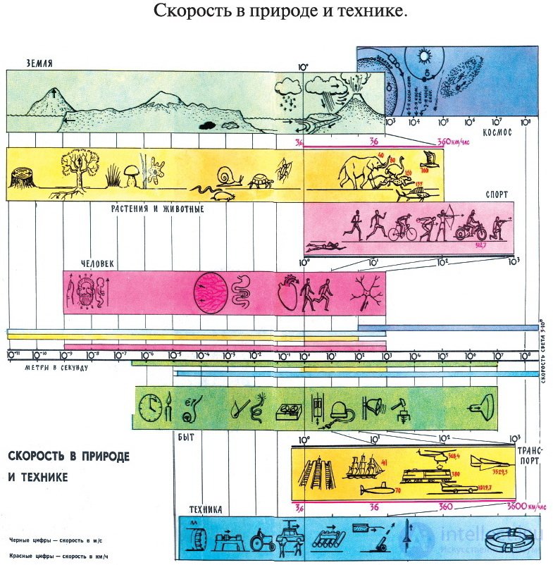
Fig. 1.3. Velocity in nature and technology
Units that are derived from the base and supplementary units by means of physical laws and definitions are called derived units.
The totality of the base, supplementary and derived units of measurement is called a system of units of measurement.
Depending on the choice of base and supplementary units of measurement, various systems of units of measurement can be constructed, differing in practical expediency and convenience of use.
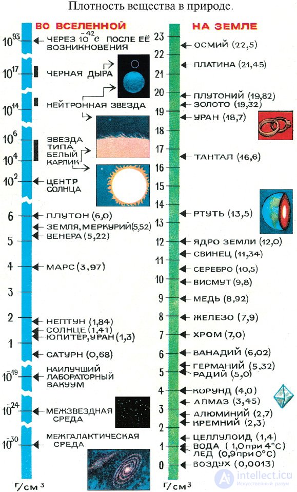
Fig. 1.4. Density of matter in nature
Let us note that in physics in general, and in theoretical physics in particular, systems of so-called natural units are widely used. We will discuss such systems of units in detail in the sections where their use is generally accepted; here we give one example to briefly explain what is meant.
The atomic system of units is introduced from the following considerations. In an atom (molecule) the main actor is the electron. This is because nuclei are several thousand times heavier than electrons and, as a rule, can be considered stationary. Indeed, the ratio of the mass of the lightest nucleus — the proton — to the mass of the electron is 1836. The main interaction determining the properties of an atom is the electromagnetic interaction, above all the electrostatic — Coulomb — interaction. Finally, an atom is a quantum object: classical (non-quantum) theory does not describe its properties. Under these conditions it is natural to assume (and this is indeed the case) that the scales of the "atomic world" are determined by such fundamental world constants as: 1) the mass of the electron  ; 2) the elementary charge — the magnitude of the charge of the electron, which is also the charge of the proton
  ; 3) the quantum constant — Planck's constant
  . In other words, it is natural to set
  , which means simply the following: we will measure the masses of all objects in electron masses, all charges — in proton charges, and all quantities with the dimension of angular momentum or of the product of energy and time — in Planck's constants. In these units the mass of the proton equals 1836, and the charge of the nucleus equals the number of protons in the nucleus, that is, the atomic number of the corresponding element. For example, the unit of length equals the radius of the first Bohr orbit of the electron in the hydrogen atom
  metres; the unit of velocity equals
  metres per second (c — the speed of light in vacuum), and the unit of energy equals
  J. Such a large unit of velocity — more than two thousand kilometres per second — and such small units of length and energy are undoubtedly extremely inconvenient in technology (see the SI system below), and even more so in everyday life, but are very convenient in the world of atoms and molecules.
Systems of units of this kind are remarkable chiefly for the fact that they are not connected in any way with the parameters of the human body (non-anthropogenic units) or other “local” — Earthly scales. By anthropogenicity we mean the following: the second — is approximately the time interval between two successive “beats” of the heart of a calmly resting healthy person, the metre — is approximately the distance from the left shoulder to the fingertips of a horizontally outstretched right arm, the sazhen — the distance between the fingertips of two horizontally outstretched arms, the kilogram — approximately the mass of two fists of an adult man. Linking one of the units of time, namely the day, to the period of the Earth's rotation is also not very good: firstly, the Earth's period of rotation changes, and secondly, other intelligent beings might not know the period of the Earth's rotation about its axis, and such a unit of time would be completely incomprehensible to them.
In the International System of Units SI (the initial letters of the French name Systeme International) the following seven units have been chosen as base units:
Base units of measurement
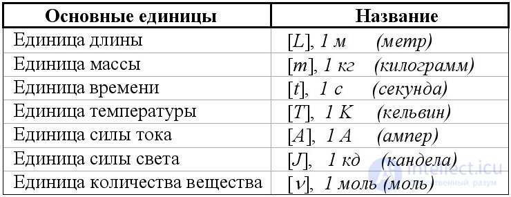
The generally accepted notation for dimensions is given in square brackets: length can be measured in metres, yards or parrots, but the notation L (from the English length) will always tell us that we are dealing with length. Similarly, the notation for the dimension of time T (from the English time) is introduced.
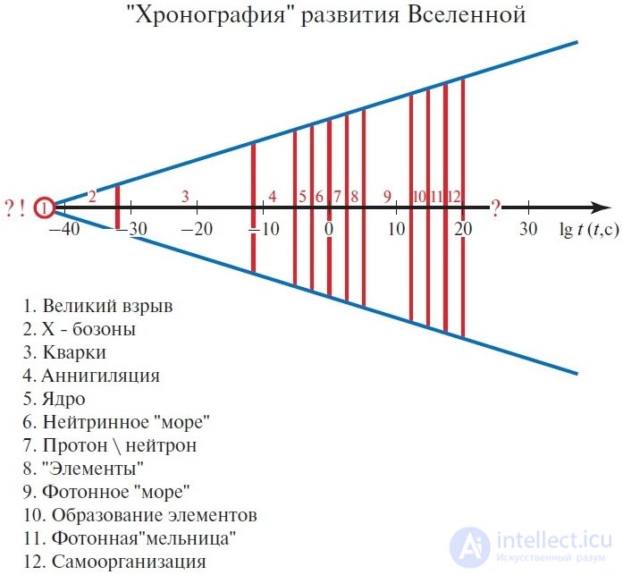
Fig. 1.5. "Chronography" of the development of the Universe
In addition to the base units, the SI system uses supplementary units.
Supplementary units of measurement
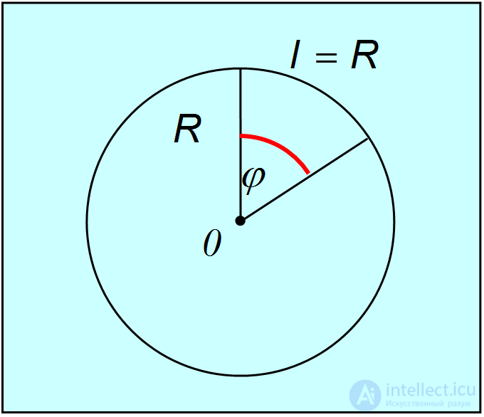
Fig. 1.6 Definition of the unit of plane angle in SI
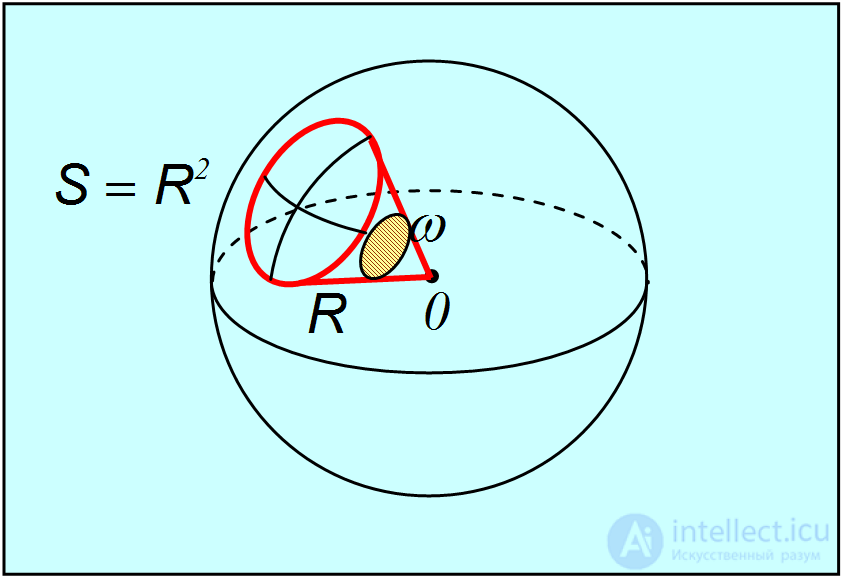
Fig. 1.7. Definition of the solid angle
 ], 1 rad (radian). The radian — is the central angle that subtends an arc whose length is equal to its radius (Fig. 1.6).
 ], 1 sr (steradian). A solid angle of 1 steradian — is the solid angle that subtends a portion of a spherical surface of arbitrary shape whose area is equal to the square of its radius (Fig. 1.7).
For simplicity, scientists strive to choose the minimal number of base quantities that allows a complete description of the physical world to be given. There is some arbitrariness in the choice of base quantities and their derivatives. We become acquainted with two of these units already from early childhood. This is natural, since all events occur somewhere and at some time. We inhabit space, which we measure in units of length. We live in time, and humanity learned to measure it in deep antiquity. Why does our world exist in time and space? We have agreed not to pose such questions, since science will not answer them anyway. But what are the properties of space and time? — this question is entirely legitimate. By studying physical phenomena, we learn the properties of space and time, and this process of learning is not yet complete.
Until recently, the international standard of the metre was considered to be the distance between two marks on a rod made of platinum alloy, kept at the International Bureau of Weights and Measures in Paris. In recent years the standard of the metre was defined by the number of wavelengths of light of a particular (orange) spectral line of the krypton isotope 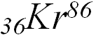 during the transition of an electron between the quantum states
  and
and  (what this is, we will learn in the final parts of the course). The metre contains 1 650 763.73 wavelengths of this spectral line in vacuum. Owing to the increased requirements for the accuracy of the length standard, in 1983 the following definition of the metre was adopted: it is the distance travelled by light in vacuum during the time
  = 1/299 792 458 seconds. In other words, it was postulated that the speed of light c is exactly equal to
  = 2.99792458 • 108 m/s. In essence, this means that instead of length, velocity was chosen as the fundamental unit, and length became a derived unit.
Fig. 1.8 shows the spatial distances characteristic of the surrounding world.
Fig. 1.8. Spatial scales in nature
The entire world accessible to our observations lies within the interval from 1026 m (the radius of the visible part of the Universe) to 10-18 m (the distances “probed” in modern experiments with elementary particles). For convenience the scale of distances  is depicted on a logarithmic scale
 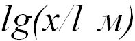 . This means that the distance 10 m on the scale corresponds to the number 1, and the distance 100 km = 100 000 m — to the number 5.
If earlier time was determined by the Sun, and the second corresponded to 1/86 400 of a mean solar day, now it is equal to the duration of 9 192 631 770 periods of oscillation of the light wave emitted during the transition between the hyperfine levels of the ground state of the caesium atom 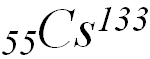 . The caesium standard is very precise: over 6 000 years two caesium clocks may diverge by only one second. There also exist even more precise clocks based on the hydrogen maser: here a discrepancy of one second accumulates over 30 million years. Perhaps the hydrogen maser will someday be adopted as the new standard of time.
Some of the time intervals encountered in nature are illustrated in Fig. 1.9.
Fig. 1.9. Time intervals in nature
The longest time about which we can obtain any information is the time of existence of the visible part of the Universe. According to current understanding, it was born as a result of the so-called Big Bang approximately 14 billion years ago (6 • 1017 s). The shortest times (10-26 s), which we encounter, correspond in order of magnitude to the time it takes light to traverse the smallest distances currently accessible to study.
He who truly understands nature
of a phenomenon must obtain
the basic laws from dimensional considerations
E. Fermi
Physical quantities are dimensional and dimensionless.
A quantity is called dimensional if its numerical value depends on the choice of the system of units.
Thus, the familiar interval of time from sunrise to sunrise we can express as 1 day, or as 24 hours, or as 1 440 min., or 86 400 s. The numbers change, but we are speaking of the same interval of time.
A quantity is called dimensionless if its value remains unchanged for any choice of the system of units.
For example, the height of Everest ( = 8 848 m) and the radius of the Earth (
 = 6 370 km) — are dimensional quantities, but their ratio is already a dimensionless quantity: regardless of the system of units
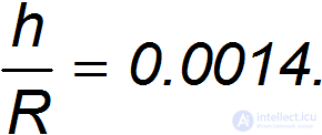
Some clarification is required for an object such as an “angle”. In the Mathematical Encyclopedia (Moscow, Soviet Encyclopedia, 1985, volume 5, p. 467) an angle is defined as follows: “An angle — is a geometric figure consisting of two distinct rays emanating from a single point. The rays are called the sides of the angle, and their common origin — the vertex of the angle”. An equivalent definition: a plane angle — is the part of a plane between two rays emanating from a single point. The radian measure of a central angle is introduced (see Fig. 1.7) as the ratio of the length of the arc of a circle that it subtends to the length of the radius of that circle:  . It is evident that a radian measure can be introduced for any angle: it is enough to place the point of a compass at the vertex of the angle, draw a circle of arbitrary radius, and calculate the ratio of the length of the arc bounded by the sides of the angle to the radius of that arc. The widely used identification of an angle (as a geometric figure) with its radian measure requires the following additional clarification: an angle is a dimensionless quantity, equal to “the ratio of the length of the arc to the radius”, but the units of measurement of this dimensionless quantity can differ. For example, to a unit of angle measurement such as the degree there simply corresponds an arc of length not equal to the radius, but to 1/360 of the length of the circumference. Another example: in marine navigation the “point” is used to measure angles, and to this unit of measurement there corresponds an arc of length equal to 1/32 of the circumference. Understanding the fact that an angle is a dimensionless quantity is very important in dimensional analysis (see below).
Dimensional quantities can be multiplied and divided by one another. Thus, the ratio of the distance travelled to the time of travel gives us a new physical quantity (velocity), whose dimension is 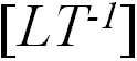 (m/s, km/h etc.). When determining the dimension of a quantity, one usually uses the dimensions of the base, not the derived, quantities. Only quantities of the same dimension can be added and subtracted (one cannot add, for example, centimetres and grams).
Any physical law and the equation describing it must not depend on the system of units we have chosen. This is natural, since a law of nature describes a relationship between quantities that existed before us, exists independently of us, and will exist after us. Whereas a system of units — is a matter of arbitrary agreement among people. From this follows a very important rule:
Both sides of any equality must have the same dimensions.
Having written down some relation, one can always check its correctness by means of dimensional analysis. Many student errors can be revealed in this way. Moreover, by fitting the dimensions one can often guess the result before carrying out detailed calculations.
Let us give an example. A car starts from rest and moves with uniform acceleration  . What speed
  will the car attain after travelling a distance
  ?
?
The application of dimensional analysis allows us to find the form of the sought relation. Velocity is a function of  and
and  . This means that it is expressed as a product of certain powers of these quantities:
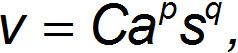
where C — is some dimensionless constant. We need to determine the exponents  and
and  . Let us write the dimensional formula for this relation:
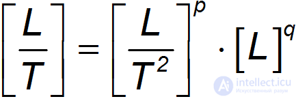
or

Since the seven base units are independent, in order for the dimensions of both sides of the equality to agree,  and
and  must satisfy the system of equations:
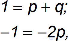
from which it follows:
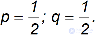
Thus, dimensional analysis leads us to the formula
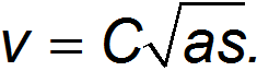
The value of the dimensionless constant C cannot be determined by this method; in the exact solution it turns out to be equal to
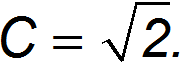
As a rule, the values of dimensionless constants in physics of the type
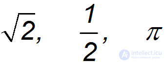
and so on, are neither too large nor too small. Therefore dimensional analysis allows us to estimate the scale of various physical quantities, in other words, to determine them by order of magnitude, or, what is the same thing, to find them accurate to a factor of order unity of the type given (for example) above.
The application of dimensional analysis requires care and a certain skill. Two pitfalls may be encountered here. The first of them — is determining the physical quantities on which the result may depend. This requires an understanding of which physical laws and phenomena are important for the system under consideration. The second pitfall — is the existence, in a given problem, of quantities that can form dimensionless ratios.
Here is another example showing how one can mislead oneself and others if one fails to take into account everything, including the dimensionless parameters of the problem. Consider a mathematical pendulum: a point particle of mass  suspended on a weightless and inextensible string of length
  in a uniform gravitational field with acceleration of free fall
  . When the string is deflected from the vertical, owing to the restoring action of the force of gravity, oscillations arise. We need to estimate the period of these oscillations
  or the frequency
  , which is related to the period by the well-known relation
  . From the three parameters
  one can form a single combination with the dimension of frequency, namely
  which does not contain the mass . Consequently, (be careful) the frequency is equal to

Using the relation between frequency and period, we obtain

These are exact expressions for the frequency and period of small oscillations of a mathematical pendulum. This fact alone gives grounds for suspicion, since the fact of smallness of the oscillations, when their amplitude  (
( — the angle of deflection of the pendulum's string from the vertical) is small:
  , was nowhere and in no way used in the estimate given above. The exact result came about by chance, because in the expression for the frequency the dimensionless coefficient was, without any grounds for doing so, set equal to unity. In reality there is a fourth, and moreover dimensionless, parameter in the problem — the amplitude of oscillation , so dimensional analysis alone can give only the following result:
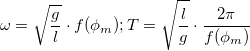
where  — some function of the amplitude of oscillation.
The function cannot be obtained from dimensional analysis. Solving the dynamical problem gives the form of this function and, in particular, its value  , which should be substituted into the last of the formulas written above for the frequency and period, on the condition that the oscillations are small.
Let us consider a more complex example: using dimensional analysis, find the drag force  exerted by a medium on a moving body. In this problem it is important from the outset to determine which quantities the sought force may depend on. What does experience tell us? The greater the velocity
  of the body's motion, the greater the drag force of the medium. So the force
  must depend on the velocity of motion. Further, bodies with a larger cross-sectional area experience greater resistance than those with a smaller one. Therefore the answer must include the cross-sectional area
  of the body. Finally, the force
  must depend on a parameter characterizing the properties of the medium. Here lies the first pitfall. Which characteristic of the medium should be chosen?
It seems natural to take the density (of air, of a liquid)  as such a parameter: the denser the medium, the greater the influence it has on the motion of the body. Based on this, we seek the drag force in the form

(the factor 2 could be absorbed into  , but we single it out for historical reasons). Force has the dimension of the product of mass and acceleration, that is
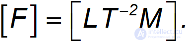
The condition that the dimensions on both sides of the equality coincide has the form:

from which follows the system of equations
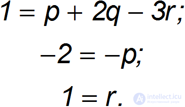
It is easy to verify that its solutions are the numbers

from which the sought formula follows
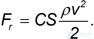
But why did we choose the density of air as the parameter responsible for the resistance of the medium? Why not instead take as such the viscosity of air  , which has the dimension
 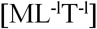 . We will get to know viscosity better later, but for now an intuitive notion suffices: at the same density a medium can be more or less viscous (jelly and compote). Then the sought force can be represented in the form

Let us write the analogous condition of equality of dimensions:

from which follows the system of equations
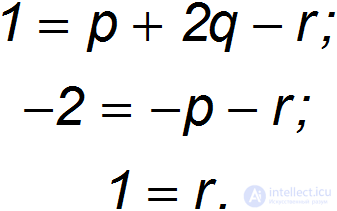
Its solution is the numbers
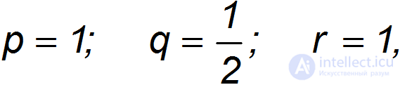
that is, the sought formula has the form:
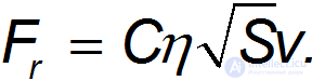
The formulas obtained for the drag force are completely different: in one of them the force depends quadratically on the velocity, in the other — linearly. So which of them is correct? This example has exposed the first pitfall: we must decide which of the two possible processes (frontal drag or viscosity of the medium) dominates in the specific problem under consideration.
Let us try to outwit the equations: let us include in the dimensional analysis both the density of air and its viscosity. We will seek the drag force in the form
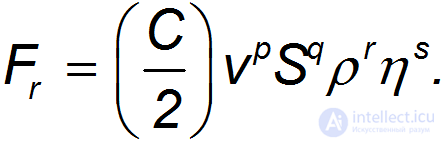
The dimensional relations take the form:


from which we obtain the system of equations:
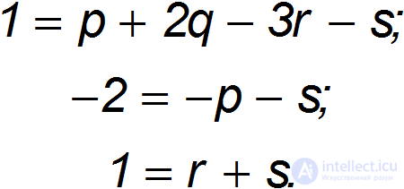
We immediately notice that the second pitfall awaits us: we have only three equations to determine four parameters. So one of them will remain undetermined. Let us try to figure out what this would mean. The last two equations allow us to express the parameters  and
and  in terms of
  :
:

Substituting them into the first equation, we obtain

from which we find
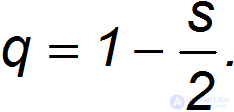
From this we obtain the drag force in the form:

The arbitrary power of the combination in the brackets indicates that this combination is dimensionless. This being so, it can be absorbed into the dimensionless quantity  , which in this case turns out not to be a constant quantity, but a function of the dimensionless parameter:
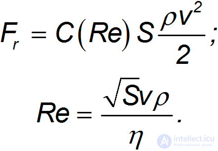
This dimensionless parameter (the Reynolds number  ) plays an important role in determining the character of the drag force. The function
 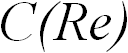 is called the drag coefficient. We will discuss the details later, but, getting ahead of ourselves, let us say right away: at low velocities the second expression for the drag force is reproduced, and at high velocities — the first formula.
This example demonstrates how to handle dimensionless combinations, should they arise in dimensional analysis.
The problems we have considered so far were solved essentially in the same, unambiguous way. Imagine that in some problem we need to find a functional relationship between N physical quantities. Assuming that this relationship has a power-law character, we can try to solve the problem by the method of dimensions. Here, if the dimensions of all N physical quantities are expressed in terms of the dimensions of the base quantities, and if in doing so N – 1 = K (where K — the number of base quantities), then there exists a unique formula giving the power-law relationship between the N physical quantities, and this formula can be found by the method of dimensions. We write the general form of the sought formula as follows: on the left-hand side stands one of the N physical quantities to the first power, and on the right-hand side — the product of powers of all the remaining (N – 1) physical quantities. The exponents are unknown. The total number of unknown exponents is also N – 1. To determine these exponents we need (N – 1) equations. We obtain each of the equations by comparing the exponents standing on the left and right for one of the base dimensions. If (N - 1) base dimensions occur in our problem, we will obtain exactly as many equations as we need. These equations are linear, and the existence and uniqueness of the solution of such a system of equations guarantees us the existence and uniqueness of the sought power-law formula.
However, there may be situations in which the rule N – K = 1 does not hold, and then we have to resort to new approaches. Let us consider a simple problem to illustrate such an approach:
What is the range of flight of a body thrown at an angle  to the horizontal with an initial velocity
  . We invite the reader to carry out the simple calculations before reading further in the textbook.
Let us try to find the relationship between S, and the angle using dimensions. The quantity sought, the range S, may depend on the initial velocity of the throw , the angle of throw, and, undoubtedly, on the acceleration of free fall  (cf. the experiment on the motion of a body thrown at an angle to the horizontal on various planets). The answer should not depend on the mass of the body — the dimension of the sought quantity does not contain the dimension of “mass”.
Thus, we have four quantities — S, ,  and
and  , between which we are trying to establish a relationship. The expressions for the dimensions of all these quantities involve only metres and seconds, i.e. N = 4, k = 2 and N – K = 2 > 1. If we write

then for the three unknown numbers  we can write only two equations. How then do we solve this problem?
Let us introduce separate units for measuring distances vertically and horizontally: distances along the horizontal axis  we will measure in “horizontal” metres —
  , and distances along the vertical axis Y — in “vertical” metres —
  . Then the dimensions are as follows:




Now for N = 4 physical quantities we already have K = 3 — the base dimensions have become 
The formula
Leads to the relation


The system of equations



has the unique solution


and we obtain the sought answer

(Compare this solution with the one you obtained in the exact calculation:  ).
).
Since we speak of measuring distances and time and have chosen the corresponding units (metres, seconds), we must agree on what these spatial and temporal distances are determined relative to. The position of an object can only be determined relative to some other bodies. We can speak of the motion of an object, that is, of a change in its position, only if we indicate the bodies relative to which this position is determined.
The bodies chosen for determining the positions of all other objects are called reference bodies.
As a reference body one can choose an arbitrary rigid body, for example, three mutually perpendicular steel rods (Fig. 1.10). Next, a point is singled out on the reference body, called the origin 0, and units of measurement of distances are chosen (in SI — metres).
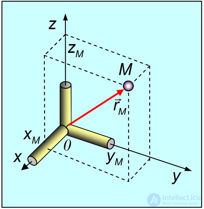
Fig. 1.10. Reference body
In everyday practice the natural reference body is our Earth. But this choice is not the only possible one. It is often convenient to use other reference bodies, for example the Sun or the stars. Relative to different reference bodies the same objects undergo different motions. It is enough to recall the dispute concerning the two astronomical systems — that of Ptolemy and that of Copernicus. Both these systems are correct, and they differ, in essence, only in the choice of reference body; Copernicus's choice of the Sun radically simplified the description of the motion of the planets, and this is precisely where his merit lies: in the Middle Ages it took considerable courage to choose the Sun, and not the Earth, as the reference body — one could have ended up at the stake.
After choosing a reference body, the position of some point M in space can be specified by means of a directed segment (the position vector  ) connecting the origin 0 to the given point M. But a vector is an abstract mathematical concept; it is filled with physical meaning when we introduce a coordinate system. This may be a Cartesian rectangular system — three mutually perpendicular axes whose point of intersection coincides with the origin. In this case the position vector is specified by three projections
  ,
,  ,
,  of the given point M onto the coordinate axes, which are called the components of the vector
  . It may be a spherical, cylindrical, or any other coordinate system, where the same position vector
  will be specified by a triplet of other numbers. The number three — this is the dimension of our space, that is, the number of independent coordinates needed to determine the position of a point. To determine the coordinates of a point one needs an instrument for determining distances, which we will conventionally call a ruler. In reality this could be a wooden school ruler, or a laser rangefinder, or anything else capable of measuring distances with the required accuracy.
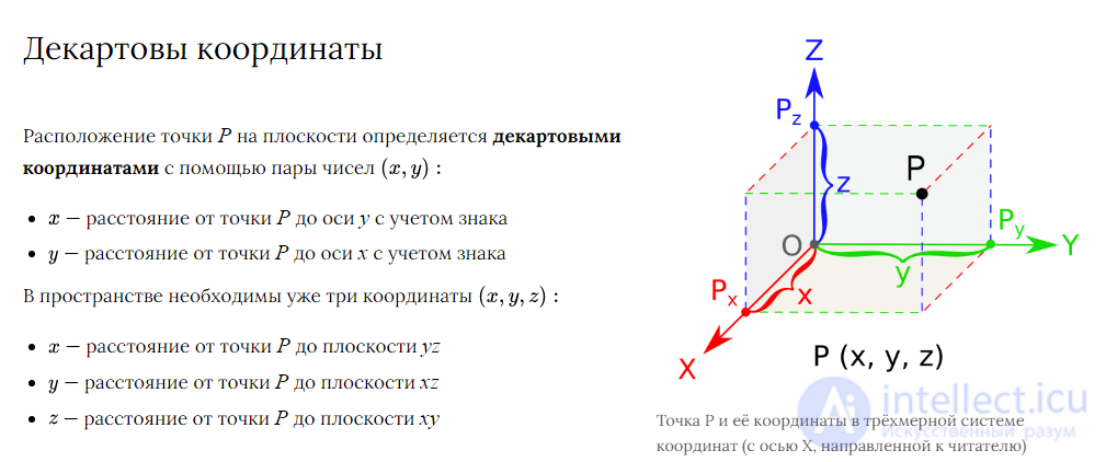
Descartes's coordinate system
To keep track of time we need some periodic processes occurring in nature or in devices created by man. Such processes (devices with such processes) we will call clocks. When solving any problem one must agree on the choice of the origin of the time count. The origin of the time count is chosen arbitrarily: one can count time from the creation of the world, or from the founding of Rome, or from the birth of Christ, or from Muhammad's flight from Mecca, and so on. As is practically always the case, the arbitrariness of the choice results in the choice being made well, less well, or altogether badly. Well or badly is determined by how simple, clear and transparent the solution of the problem under consideration turns out to be. Unlike three-dimensional space, time is one-dimensional, so in addition to the origin of the time count it suffices to choose only the units of measurement (seconds).
To keep track of time we need some periodic processes occurring in nature or in devices created by man. Such processes (devices with such processes) we will call clocks. When solving any problem one must agree on the choice of the origin of the time count. The origin of the time count is chosen arbitrarily: one can count time from the creation of the world, or from the founding of Rome, or from the birth of Christ, or from Muhammad's flight from Mecca, etc. As is practically always the case, the arbitrariness of the choice results in the choice being made well, less well, or altogether badly. Well or badly is determined by how simple, clear and transparent the solution of the problem under consideration turns out to be. Unlike three-dimensional space, time is one-dimensional, so in addition to the origin of the time count it suffices to choose only the units of measurement (seconds).
A reference body, equipped with a coordinate system and clocks, is called a frame of reference..
An example of a frame of reference is shown in Fig. 1.11.
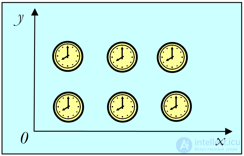
Fig. 1.11. Frame of reference
A frame of reference is often identified with a coordinate system, which practically never leads to misunderstandings. However, one must understand that these are still not the same thing: with the same reference body, ruler and clocks, the coordinate system can be Cartesian, spherical, or any other.
In classical mechanics, which was formulated in its modern form by I. Newton, an absolute character of space and time is assumed. In other words, in classical mechanics it is considered that the measured distances and time intervals do not depend on the choice of frame of reference. Say, if in a frame of reference associated with the Earth the distance from Moscow to Tallinn is 860 km, then it is assumed that the result of measurements made relative to a frame of reference associated with the stars will be the same. These propositions, which seem so natural, follow, strictly speaking, only from our practical experience, limited to comparatively small distances, times and low velocities. Subsequently they were revised by the theory of relativity.
As is known, there are scalar quantities, which have no direction, and there are vector quantities, to which, besides magnitude, some direction is assigned. Time — is a scalar quantity, while position in space must be specified by vectors. It is not enough to say that a lecture will take place 860 km from Tallinn. This information is not enough to find out exactly where: in Moscow or, say, in Copenhagen. From this it is clear that vectors must play an important role in physics. It is no accident that vector calculus acquired its modern form precisely thanks to the works of physicists (J. Gibbs). Besides length and direction, for vectors the operations of multiplying a vector by a real number and of adding vectors are defined, that is, a vector algebra is specified.
The use of vector calculus is convenient in that many relations are obtained in a general, compact form and can be transformed without much difficulty into the corresponding relations for any coordinate system. Relations between vectors remain unchanged when the origin is changed or another coordinate system is chosen. In this section we will recall some rules of vector algebra. Since we are now dealing with physics, we do not strive for exact mathematical proofs.
Let us be given some Cartesian rectangular coordinate system. Any vector A can be specified by three components  — the projections of the vector onto the axes
  ,
,  ,
,  . In what follows we will use both generally accepted notations for vectors, either setting the corresponding letter in bold type, or placing an arrow over it:
The magnitude of vector A (or its length) is called the number:

The length of a vector does not change under rotations of the coordinate system.
The product of vector A and the number  is a vector

whose projections are defined as

From this it follows, first, that the length of vector B is equal to the length of vector A, multiplied by the absolute value of the number 

Second, the vectors A and  A are collinear and have the same direction if
  >0, and the opposite direction if
  <0.
<0.
The sum of two vectors A and B is called the vector c

whose components are defined as the sum of the components of the addends

From this follows the geometric representation of the sum of vectors — the parallelogram rule or the triangle rule (Fig. 1.12).
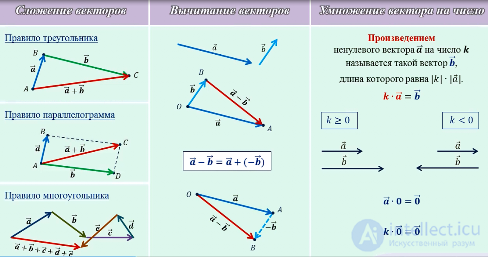
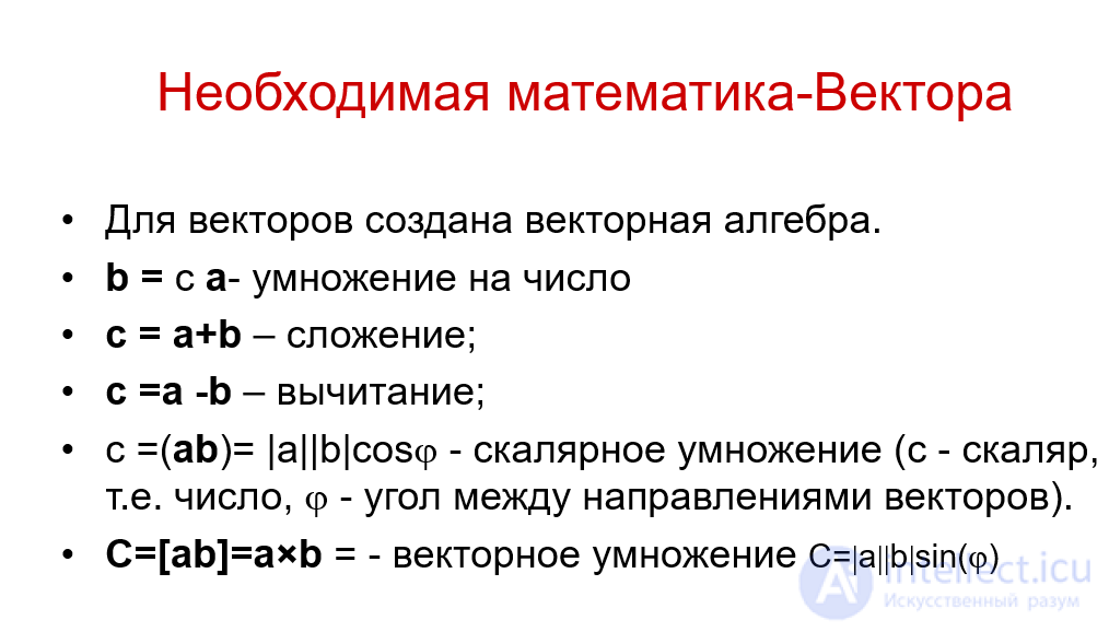
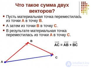
Fig. 1.12. Addition of two vectors
Similarly for the subtraction of vectors

where

The rule for subtracting vectors is illustrated in Fig. 1.13.
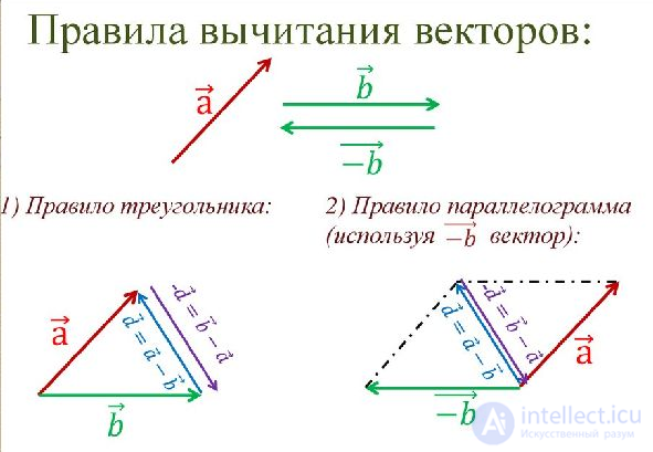
Fig. 1.13. Subtraction of vectors
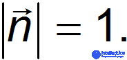
A unit vector n — is a vector with length equal to unity
The unit vector nA in the direction of some vector a is equal to

Unit vectors along the positive directions of the axes  , ,
, ,  of the coordinate system play a special role.
Unit vectors along the positive directions of the axes  ,
,  ,
,  of the coordinate system

are called orts (unit basis vectors).The set of orts constitutes the basis of the given coordinate system.
Sometimes the axes are marked with numbers (1,2,3) or with indices corresponding to the axes (x,y,z) denoted as follows
 or
or 
Any vector a can be represented as an expansion in the basis

Fig. 1.14 shows the expansion of a vector along the coordinate axes
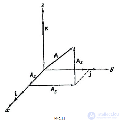
Fig. 1.14. Expansion of a vector along the coordinate axes
The scalar (dot) product of two vectors a and b — is a number equal to the sum of the products of the corresponding projections of the vectors — the factors

From this it follows that the scalar product of a vector with itself is equal to the square of the length of the vector

The second consequence: the scalar product is commutative, that is

The relation also holds

The scalar product does not depend on rotations of the coordinate system. The system can be rotated so that both vectors lie in the plane  and the axis
  is directed along vector a. In this rotated coordinate system the factor vectors have the following projections:

Therefore the scalar product can also be represented in the form

Here  — is the angle between vectors a and b.
If the vectors are orthogonal, that is
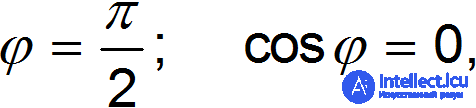
then the scalar product is equal to zero:
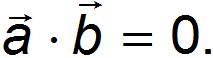
Conversely: if the scalar product is equal to zero, then either one of the factors is a vector of zero length, or they are orthogonal.
Fig. 1.15. Scalar product
Let us give an example of using the scalar product (Fig. 1.16). Let
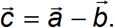
Let us square both sides of the equality:

This is — the so-called law of cosines; in the particular case of a right triangle 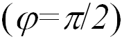 the Pythagorean theorem follows from it.
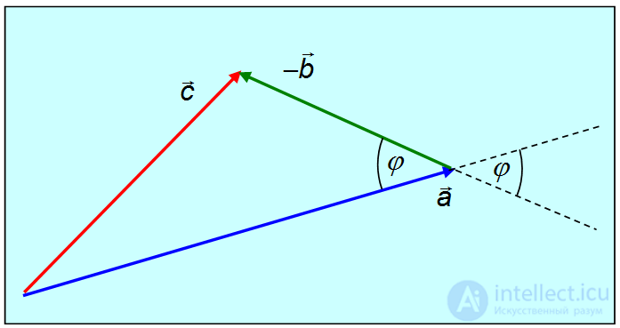
Fig. 1.16. Law of cosines
The vector (cross) product of two vectors a and b — is a vector c, whose components are equal to
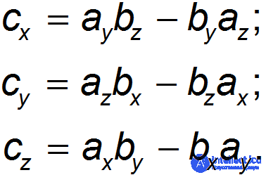
From this it follows that the expansion of the vector product in the basis can be represented as a determinant
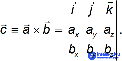
(1.5.1)
To denote the vector product either an oblique cross between the factors is used, or the factors are placed, separated by a comma (the comma is optional if it is clear without it where the first factor ends and the second begins), in square brackets.
It is also evident that in the vector product the order of the factors matters

The relation holds

To understand where the vector product is directed and what its length equals, let us again rotate the coordinate system so that the plane of the axes  coincides with the plane of vectors a and b and the axis
  is directed along vector a. Then

Substituting these values into the determinant (1.5.1) for the vector product, we obtain
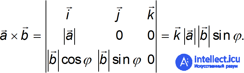
This means that the length of the vector product is equal to
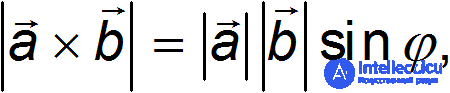
and it is orthogonal to both factors a and b, with its direction determined by the right-hand screw rule.
If a right-hand screw is turned from the first factor vector to the second along the shortest path, then this screw moves in the direction of their vector product.
The application of the right-hand rule is illustrated in Fig. 1.17.
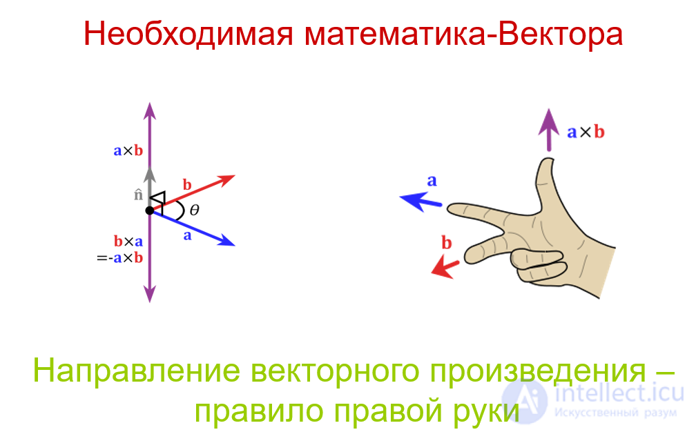
Fig. 1.17. The right-hand rule for determining the direction of the vector product
\
If the factors of the vector product are collinear ( ,
,  ;
; 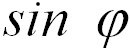 = 0), then the vector product is equal to zero. Conversely, from the vector product being equal to zero it follows that either the factor vectors are collinear, or one of the vectors is equal to zero.
Division by a vector is not defined.
The derivative of vector a — is a vector whose components are equal to the derivatives of the corresponding components of vector a.
Let, for example, vector a depend on time t. Then

The derivatives of scalar and vector products look as usual:
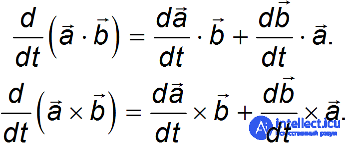
Let us emphasize that in the expression for the derivative of the vector product the original order of the factors must be preserved.
Required mathematics — Differentiation
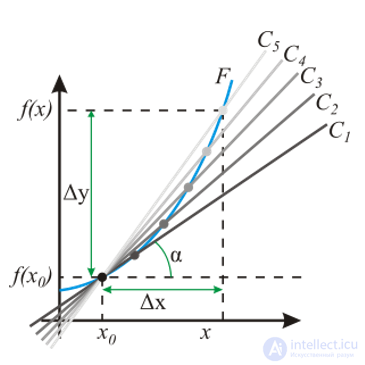
Definition of the derivative
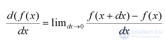
Geometric meaning of the derivative – the tangent at point x
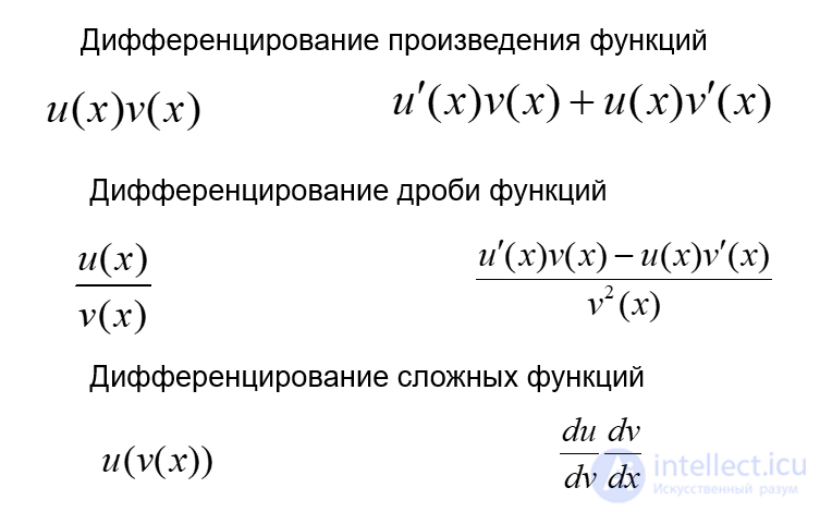
Rules of Differentiation
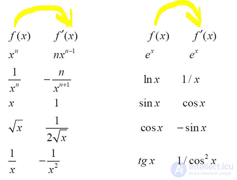
Examples of derivatives
Required mathematics — Integration
Definition of the integral
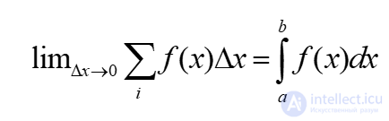
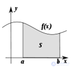
The definite integral as the area under a curve
Calculation of the definite integral
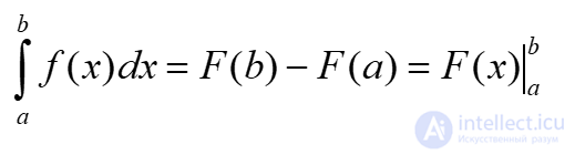
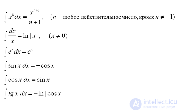
Table of indefinite integrals

Comments