
Lecture
In the following chapters we consider systems moving at non-relativistic speeds. Therefore we return again to the equations of classical non-relativistic mechanics, now aware of the limited range of their applicability.
In topic 2.8 we considered the kinematics of a rigid body and discussed two types of motion: translational, when all points of the body describe identical trajectories, and rotational about an axis, when the points of the body move in parallel planes and describe circles centred on the axis of rotation.
Any motion of a rigid body reduces to translational and rotational motion. Arbitrary motion can be represented as a superposition of the translational motion of the whole body, characterized by the motion of some point (for example, the centre of mass), and rotation of the body about this point (that is, about the axes passing through it).
We will begin the study of rigid body dynamics with the simplest case — rotation about a fixed axis, and finish by discussing the operating principle of the wheel — humanity's most ingenious invention.
The motion of a point particle is characterized by displacement, velocity, and acceleration. But when a rigid body rotates, all its elements have different displacements and different velocities. It is convenient to find variables that are the same for all elements of the rigid body. We in fact already know them — the angle of rotation, angular velocity, angular acceleration. Accordingly, in studying rotational dynamics, instead of momentum and force we will operate with their angular analogues — angular momentum and torque.
Equation of motion. In topic 4.8 the equation of motion of a system of point particles was derived in the form

where the angular momentum and torque were defined as
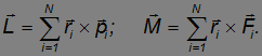
The internal forces between the bodies of the system, recall, dropped out of the equations of motion. An absolutely rigid body can be regarded as a system of particles (point particles) with unchanging distances between them. Therefore the equations written above apply to a rigid body, and the constancy of the distances between its points allows the rotation of the body about a fixed axis to be characterized by a single coordinate — the angle of rotation. Therefore we can simplify the equation of motion given above. First of all, we are not interested at the moment in the stresses arising in the axis. Moreover, to describe rotation it is sufficient to consider the projections of the angular momentum and torque vectors onto the axis of rotation.
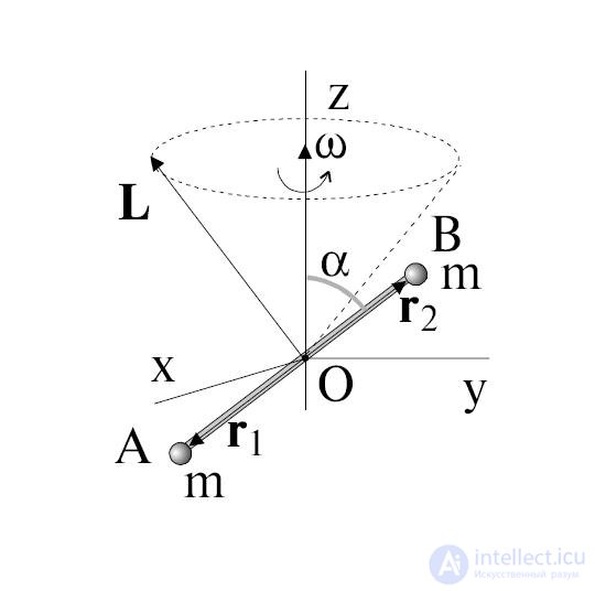
Fig. 7.1. Angular momentum L of two balls of mass m connected by a rod. The whole system rotates about the z axis with angular velocity ω
Direct the z axis along the axis of rotation and single out in the rigid body an element of mass  , whose position is characterized by the position vector
  (fig. 7.2).
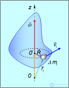
Fig. 7.2 Rotation of a rigid body about a fixed axis 0z
The angular momentum of this element is
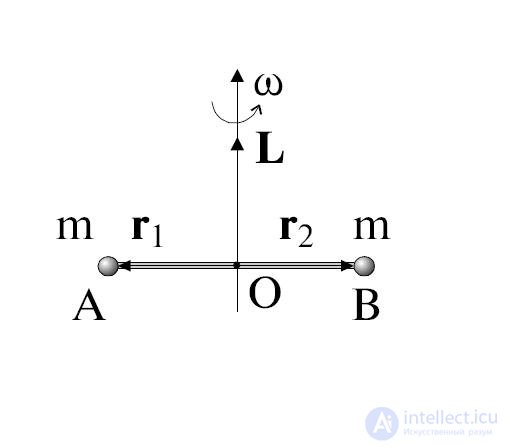
Fig. 7.3. The angular momentum of the system is directed along the axis of rotation.
The position vector can be represented as the sum of its projections onto the z axis and the xy plane:
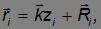
where the vector  lies in the plane of rotation and is directed from the axis to the selected element (see fig. 7.1). We have:

The first term is a vector directed opposite to Therefore it makes no contribution to the z-component of the angular momentum. The second term is a vector directed along the z axis. Since

and

we can write:

Summing over all elements of the body, we obtain
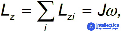
where
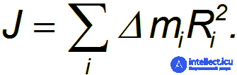
The quantity  is called the moment of inertia of the body.
When speaking of the moment of inertia, it is always necessary to indicate with respect to which axis of rotation it is defined (in this case — the z axis). The moment of inertia of the same body with respect to a different axis will take a different value. Only the general rule for computing it is preserved: take the sum, over the elements of mass making up the body, of each multiplied by the square of the distance of that mass element from the axis of rotation.
In the case of a continuous mass distribution with density  the sum is replaced by an integral over the entire volume of the body:
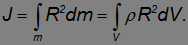
If the body is homogeneous, its density is constant at all points and can be taken outside the integral sign.
We now write the equation of motion in projection onto the z axis:

If the moment of inertia does not depend on time, then only the angular velocity needs to be differentiated, and as a result we obtain the fundamental equation of the dynamics of rotational motion of a rigid body in the form
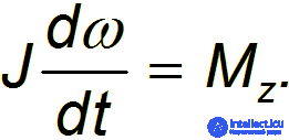
The derivative of the angular velocity with respect to time is the angular acceleration

Video 7.1. The fundamental equation of the dynamics of rotational motion. A demonstration of the relationship it implies between angular acceleration, torque and moment of inertia
Let us now consider the moment of the external forces. We decompose the force  into a vector in the direction of the z axis and a vector orthogonal to it:
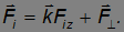
Using again the analogous decomposition of the position vector
we obtain for the moment of the external forces  :
:
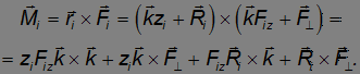
The first term is equal to zero. The next two contain the unit vector — vector k, directed along the 0z axis and, consequently, make no contribution to the projection  . Both vectors

lie in the xy plane and, consequently, the last term is directed parallel to the 0z axis. If  — is the angle between these vectors, then

where  — is the lever arm of the force (see topic 4.8). The force

should be understood here in the algebraic sense: it enters with a minus sign if the force decelerates the rotation.
Moment of inertia. Let us find the moments of inertia for the simplest (geometrically regular) shapes of a rigid body whose mass is uniformly distributed over its volume.
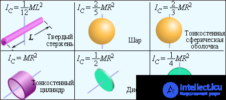
Fig. 7.4. Moments of inertia of various bodies
1. Moment of inertia of a hoop with respect to an axis perpendicular to its plane and passing through its centre.
The hoop is considered infinitely thin, that is, the thickness of the rim can be neglected in comparison with the radius  . Since in this system all masses are at the same distance from the axis of rotation,
  can be taken outside the integral sign:

where  — is the total mass of the hoop.
2. Moment of inertia of a disc with respect to an axis perpendicular to its plane and passing through the centre.
The disc is considered infinitely thin if its thickness is much less than the radius . The moment of inertia, by definition, is an additive quantity: the moment of inertia of a whole body equals the sum of the moments of inertia of its parts. Let us divide the disc into infinitely thin hoops of radius  and width
  (fig. 7.5).
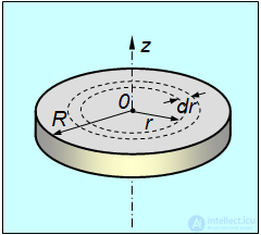
Fig. 7.5 Calculating the moment of inertia of a disc about the z axis, perpendicular to its plane and passing through the centre
The surface area of the hoop equals the product of its circumference by its width:  . Since the mass m of the disc is uniformly distributed, the mass per unit area equals
  , so that the mass of the hoop equals

We already know the moment of inertia of a hoop:
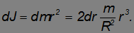
It remains to sum the moments of inertia of all such hoops:

The same result is obtained for the moment of inertia of a cylinder of finite length with respect to its longitudinal axis.
3. Moment of inertia of a sphere with respect to its diameter.
Let us proceed in an analogous manner: “slice” the sphere into infinitely thin discs of thickness  , located at a distance z from the centre (fig. 7.6).
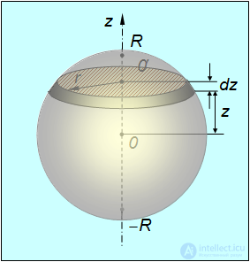
Fig. 7.6. Moment of inertia of a sphere with respect to its diameter
The radius of such a disc is
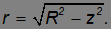
The volume of the disc  equals its area multiplied by its thickness:
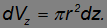
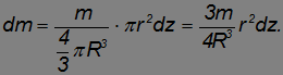
We find the mass of the disc  by dividing the mass of the sphere by its volume
  and multiplying by the volume of the disc:
The moment of inertia of a disc was found above. Applied to this case it equals

The moment of inertia of the sphere is found by integrating over all such discs:
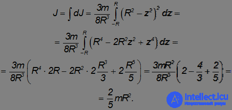
4. Moment of inertia of a thin rod with respect to an axis passing through its midpoint perpendicular to the rod.
Let the rod have length  . We direct the x axis along the rod. By condition, the origin of coordinates is at the centre of the rod (fig. 7.7).
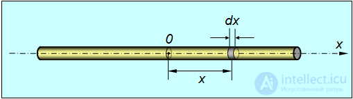
Fig. 7.7. Moment of inertia of a thin rod with respect to an axis passing through its midpoint perpendicular to the rod
Let us take an element of the rod of length  , located at a distance x from the axis of rotation. Its mass equals

and its moment of inertia
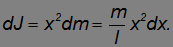
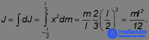
From this we find the moment of inertia of the rod:
Steiner's theorem. In the examples given, the axes pass through the centre of mass (centre of inertia) of the body. The moment of inertia with respect to other axes of rotation is determined in accordance with Steiner's theorem (the parallel axis theorem):
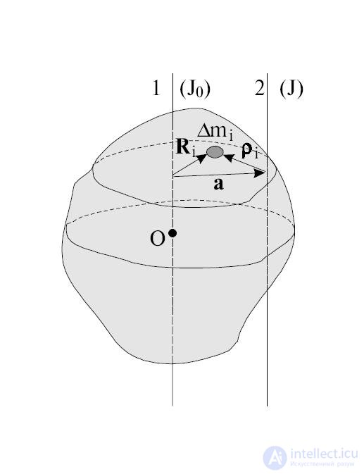
Fig. 7.8. Toward the derivation of Steiner's theorem
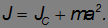
The moment of inertia of a body with respect to an arbitrary axis equals the sum of the moment of inertia JC with respect to a parallel axis passing through the centre of inertia of the body, and the quantity ma2 — the product of the mass of the body and the square of the distance from the centre of inertia of the body to the chosen axis, that is
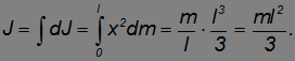
Let us first demonstrate the application of Steiner's theorem. We calculate the moment of inertia of a thin rod with respect to an axis passing through its end, perpendicular to the rod. Direct calculation reduces to the same integral that arose when calculating the moment of inertia of the rod with respect to the axis passing through its midpoint, but taken with different limits:
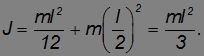
The distance to the axis passing through the centre of mass is a = l/2. By Steiner's theorem we obtain the same result:
The derivation of Steiner's theorem is illustrated in fig. 7.8, 7.9
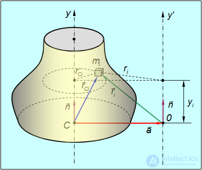
Fig. 7.9. Toward the derivation of Steiner's theorem
Let one axis pass in the direction of the unit vector n through the centre of mass C of the rigid body (system of bodies), and another — parallel to it through some point 0. From the centre of mass, in the direction of the second axis, we draw a vector a orthogonal to the axes, which determines the position of point 0. The position vectors of some element of the system of mass  relative to points C and 0 we denote
  and
and  , respectively. The moment of inertia of this element with respect to axis C is

where  — is the distance of the element from the axis. By the Pythagorean theorem (see fig. 7.9).
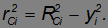
The leg  equals the projection of the vectors and onto the axis of rotation, that is

Using these expressions and summing over all elements of the system, we find the moment of inertia with respect to the axis passing through point C, and, in an analogous manner, the moment of inertia with respect to the parallel axis passing through point 0:
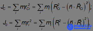
Here the expression for  is obtained from
  by a simple replacement of with .
As seen from fig. 7.9, the vectors and are related to each other:
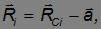
moreover
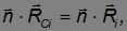
since the vectors n and a are orthogonal and their dot product

Then we can transform the expression for :
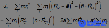
The first term on the right-hand side — is the moment of inertia with respect to the axis passing through point C. The third term equals  , where

— is the total mass of the system.
The second term equals zero, since it is proportional to the position vector of the centre of inertia relative to the centre of inertia itself. Finally:
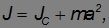
which is what we set out to prove.
Steiner's theorem relates moments of inertia with respect to parallel axes. Sometimes another theorem, relating moments of inertia with respect to three mutually perpendicular axes, turns out to be useful. However, this theorem applies only to flat figures whose thickness can be neglected in comparison with their dimensions in the two other directions. So, the theorem on the moments of inertia of flat figures:
If, through an arbitrary point 0 of a flat figure, an axis orthogonal to the figure is drawn, then the moment of inertia with respect to this axis equals the sum of the moments of inertia with respect to two mutually perpendicular axes lying in the plane of the figure and passing through this same point 0.
In other words, we take an arbitrary point 0 on the figure and draw coordinate axes so that 0x and 0y lie in the plane of the figure. Then, according to the theorem, the moment of inertia with respect to the axis 0z equals the sum of the moments of inertia with respect to the axes 0x and 0y:
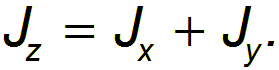
Here the arrangement of the axes 0x, 0y can be arbitrary; the main thing is that they lie in the plane of the figure (fig. 7.10).
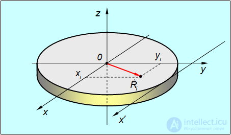
Fig. 7.10. Moments of inertia of a flat figure with respect to mutually perpendicular axes
From the figure it is seen that
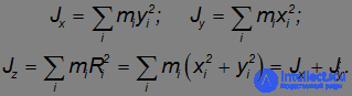
which is what we set out to prove.
Let us find, for example, the moment of inertia  of a disc with respect to its diameter. Two orthogonal diameters of the disc are equivalent, therefore

According to the flat figure theorem
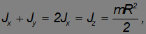
from which

Now we can apply Steiner's theorem to find, for example, the moment of inertia  with respect to the axis
  , parallel to the diameter and passing through the edge of the disc (see fig. 7.10):

Let us determine the work done by external forces when a rigid body rotates about a fixed axis 00. The elementary work done in moving an element of mass  equals:

where  — is the tangential component of the external force
  acting on the element of mass (fig. 7.11).
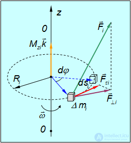
Fig. 7.11. Work of forces when a rigid body rotates
Let us recall the decomposition of the force
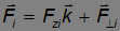
into a vector parallel to the axis of rotation (let us take it as the z axis), and a vector orthogonal to it. During rotation the displacement is directed tangentially to the trajectory, that is, firstly, it lies in the plane of rotation. It follows that the force  , directed along the axis of rotation, does no work. Secondly, the displacement is orthogonal to the radius of the circle described by the given element. The projection of the external force onto the plane of rotation can in turn be decomposed into the terms
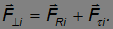
One of them ( ) is directed along the radius; it is orthogonal to the displacement and therefore also does no work. Work is done only by the projection of the force onto the tangential direction
  , which appears in the expression for the elementary work.
The path  can be written as

Thus,
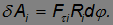
Note that

where  — is the lever arm of the force introduced above.
Consequently, we have expressed the elementary work done in moving an element of mass through the projection of the moment of the external force onto the axis of rotation:
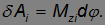
Therefore the elementary work done in rotating the whole rigid body equals

where M is the total moment of all the external forces, and the vector  is directed along the axis of rotation according to the right-hand rule.
For the total work over time  we can write:
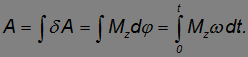
The projection of the moment of the external forces can be expressed through the angular acceleration, using the fundamental equation of the dynamics of rotational motion

Then, taking into account  , we obtain

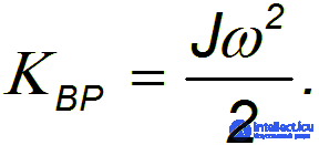
According to the law of conservation of energy, the work  equals the increment
  of the kinetic energy of the rigid body. Thus, the kinetic energy of a rotating body equals
Between the quantities describing translational and rotational motion there exists an analogy, which makes it easier to learn and remember these quantities and the relations between them (see the table).
Table
Analogy between translational and rotational motion
| Translational motion | Rotational motion |
|---|---|
Displacement  |
Rotation |
Velocity  |
Angular velocity  |
Acceleration  |
Angular acceleration  |
Mass  |
Moment of inertia  |
Momentum  |
Angular momentum  |
Force  |
Torque  |
Equation of motion  |
Equation of motion  |
Work  |
Work  |
Kinetic energy  |
Kinetic energy
|
Let us now consider the plane motion of a rigid body, that is, motion in which the points of the body describe trajectories lying in parallel planes. An example of such motion — the rotation of a car's wheel as it moves in a straight line. One can take any point 0 of the body and mentally draw through it an axis of rotation perpendicular to the planes in which the trajectories of the body's points lie. Then the axis of rotation will move translationally, remaining parallel to itself at all times.
Video 7.2. Plane motion of a rigid body in a uniform gravitational field. Flight of a flat cardboard figure
Accordingly, the velocity  of an elementary mass
  of the rigid body is made up of the velocity
  of the translational motion of point 0 and the linear velocity of rotation about the (mentally drawn) axis associated with it:
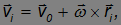
where  — is the position vector determining the position of the elementary mass relative to point 0.
The kinetic energy of the elementary mass is then equal to:
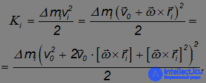
The vector product

has a magnitude equal to  , where — is the distance of the mass from the axis of rotation. Consequently, the third term in the brackets equals
  . The second term, representing a scalar triple product of vectors, does not change under cyclic permutation of the factors:

As a result we obtain the following expression for the kinetic energy of an element of the rigid body

To find the kinetic energy of the body we sum over all elementary masses:

The sum of the elementary masses

is the mass of the rigid body. The expression
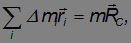
where  — is the position vector of the body's centre of mass relative to point 0.
Finally,

— is the moment of inertia of the body  relative to the axis of rotation. Therefore, for the kinetic energy of a rigid body we can write the formula:

Since the choice of the imaginary rotation axis is entirely up to us, we shall simplify the resulting expression by taking the centre of mass of the body as point 0. Then = 0, and the kinetic energy of a body in plane motion equals
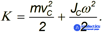
Here  — is the velocity of the centre of mass, and
  — is the moment of inertia about the axis passing through the centre of mass and orthogonal to the plane in which the trajectories of the body's points lie. Thus, the kinetic energy of a rigid body in plane motion consists of the energy of translational motion at a speed equal to the speed of the centre of mass, and the energy of rotation about the axis passing through the body's centre of mass.
The motion of a rigid body is determined by the external forces acting on the body and the moments of these forces
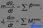
The index  in the notation for the moment of the external force denotes the projection of the moment onto the axis of rotation.
In the following examples we deal with plane motion.
Video 7.3. How the behaviour of cylinders on an inclined plane depends on the way mass is distributed through their volume
Example 1. A round homogeneous body (hoop, cylinder, sphere) of radius  and mass
  rolls without slipping down an inclined plane at an angle
  to the horizontal from a height
  (Fig. 7.12). The initial velocity of the body is zero. Let us find the velocity of the centre of mass of each body at the end of the descent.
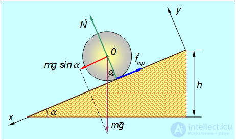
Fig. 7.12. A body rolling down an inclined plane
This problem can be approached in two ways.
1st method. By the problem's condition, the body rolls without slipping. This condition is used twice here. The friction force between the body and the plane acts at the point of contact and, in the absence of slipping, does not exceed its maximum value:
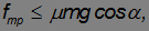
where  — is the coefficient of sliding friction.
It is convenient to direct the coordinate axes as follows: the x axis — along the direction of motion, the y axis — perpendicular to the inclined plane. The body moves under the action of three forces: the force of gravity  , the friction force
  and the normal force
  , so that the equation of translational motion of the body's centre of inertia has the form:
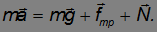
Along the y axis the body does not move. Projecting the equation of motion of the centre of mass onto the y axis, we obtain the following relation for the normal force:

The projection of the equation of motion onto the x axis gives:

Since the linear velocity of the points of contact of the cylinder with the inclined plane is zero (again using the no-slipping condition), the velocity (acceleration) of the translational motion is related to the angular velocity (angular acceleration) of the body by the usual relations:

In addition to translational motion, the body also rotates. It is convenient to describe the rotation relative to the z axis passing through the centre of mass of the cylinder.
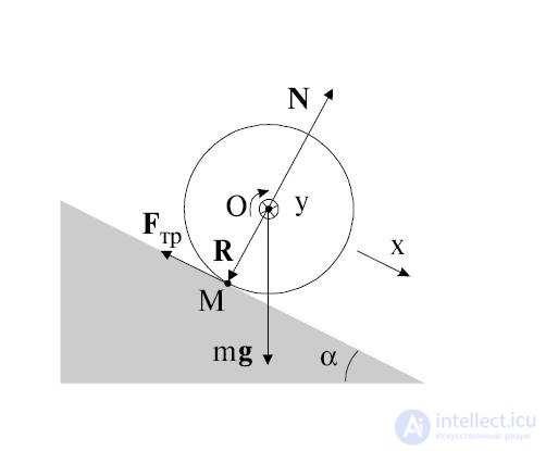
This choice is due to the fact that the lines of action of the force of gravity and of the normal force of the plane pass through the axis of rotation, and hence the moments of these forces are equal to zero. Thus, the cylinder rotates only under the action of the friction force, and the equation of rotational motion has the form:

Thus, we obtain a system of 4 equations describing the translational and rotational motion, together with an additional inequality expressing the law of friction. Solving the system of equations, we find:
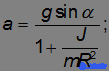
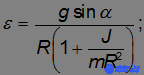
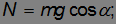
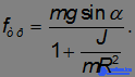
The greater the moment of inertia about the axis passing through the centre of mass, the smaller the acceleration of the body. We have already obtained the answer to one of the questions of the problem: the sphere will move faster than the cylinder, and the cylinder — faster than the hoop. Substituting the solution for the friction force into the inequality expressing the law of friction, we find the condition under which slipping will be absent:
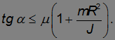
The meaning of this condition is simple: the incline must not be too steep.
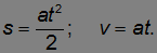
So, the centre of mass of the body moves along the plane with constant acceleration a, so that the dependence of the distance travelled and the velocity on time has the form:
From this follows the relation between the velocity and the distance travelled:

By the end of the descent the body covers a distance

so that its velocity reaches the value
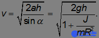
Substituting here the moments of inertia of the hoop ( ), the cylinder (
 ) and the sphere (
 ), we find respectively:
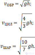
2nd method. Let us use the law of conservation of total energy. At the end of the descent the body acquires kinetic energy

This kinetic energy has been acquired at the expense of the potential energy  . From this follows the expression found above for the velocity of the body at the end of the descent. This method is much shorter, but it does not allow us to learn the details of the process: the forces acting on the body, and so on.
In the example considered above we assumed the case in which slipping was absent. This allowed us to state the simple relation ( ) between the angular and linear velocities of the body and its radius. The force of static friction was found here as a result of solving the equations of motion. In the case when the body moves with slipping, there is no known relation beforehand between the linear and angular velocities. However, we do know the friction force in advance: since the point of contact of the body with the surface slides over the surface, the friction force is a force of sliding friction, whose magnitude is related to the normal force by the Amontons–Coulomb law.
As has already been said, friction forces are directed so as to oppose the relative slipping of bodies in contact. This possible slipping is often confused with the translational motion actually taking place. It must be clearly understood that it is not rare for the friction force not to decelerate the body but to accelerate it, that is, to act in the direction of its motion. The best-known example is a car starting to move. The wheels begin to rotate and slip backward against the ground. Correspondingly, the friction force is directed forward, and it is precisely this force that makes the car start moving. To get better acquainted with such cases, let us consider an example.
Example 2. A circus performer throws onto the arena a hoop of mass and radius , which starts rolling in the horizontal direction with velocity  (Fig. 7.13). At the same time the hoop is given reverse spin with angular velocity
  . Let us find at what angular velocity the hoop, after stopping, will roll back toward the performer, as well as the final velocity
  of the hoop's translational motion.
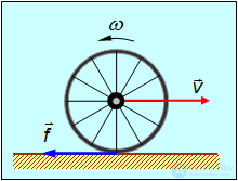
Fig. 7.13. Motion of a hoop with reverse spin
With the hoop spinning in reverse, its point of contact with the arena moves forward both because of the rotation and because of the translational motion of the hoop. Therefore slipping inevitably occurs, and hence the friction force reaches its maximum value. It decelerates both the translational motion and the rotation of the hoop. It may happen that the translational motion of the hoop is stopped at a moment when it still retains its reverse spin. After that the friction force begins to accelerate the hoop toward the performer. This acceleration ceases when the tendency to slip disappears, after which the hoop begins to roll back uniformly with some steady-state velocity . It may, however, also happen that the reverse spin is stopped first, and then the hoop retains its forward translational motion, having changed the direction of its rotation to the direct one. To distinguish these two cases, qualitative reasoning is not sufficient, and we turn to the formulas.
Let us direct the OX axis to the right (in the direction of the red arrow in Fig. 7.13), the axis of rotation OZ toward us (see the next example, where it is more convenient to direct this axis away from us, that is, into the drawing), that is, in the direction of the “reverse” spin, and the OY axis as usual, upward. We shall represent the plane motion of the hoop as a superposition of its translational motion together with the centre of mass (the geometric centre, since the hoop is assumed to be homogeneous). Let us project the linear and angular velocities onto the corresponding axes. Then, as long as the friction force is a sliding-friction force and is directed to the left, the equations of motion have the form

(7.3.1)

(7.3.2)
Equation (7.3.1) describes the motion of the centre of mass of the hoop, while equation (7.3.2) describes its rotation about the axis passing through the centre of mass in the reference frame in which it is at rest (the centre-of-mass frame). In (7.3.2) it is taken into account that the moment of inertia of a homogeneous hoop about its axis of symmetry equals  . After elementary integration we obtain

(7.3.3)
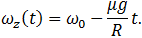
(7.3.4)
The translational motion will cease, that is,  will become equal to zero, at the moment of time

(7.3.5)
The rotation will cease, that is,  will become equal to zero, at the moment of time
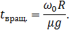
(7.3.6)
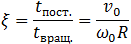
Their ratio
(7.3.7)
can be arbitrary in view of the independence of the initial translational velocity  and rotational velocity
  .
.
For further analysis let us introduce the velocity  of the lowest point of the hoop — the point of it that touches the surface of the arena. Let us note here already that the condition for the disappearance of slipping is that the velocity of precisely this point vanishes, because the velocity of the corresponding point on the surface of the arena (the one touched by the hoop) is, obviously, in our reference frame, where the arena is stationary, equal to zero. The absence of slipping is precisely the immobility of these two points relative to each other. With the chosen direction of the OZ and OX axes, we have

(7.3.8)
If  , then the translational motion of the hoop will cease first. At the moment of time
  the velocities (7.3.3) and (7.3.8) will have the values
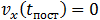

The lowest point of the hoop, owing to the continuing rotation, will still be sliding relative to the arena to the right (to the right in Figure 7.13), the sliding friction force will keep its magnitude and direction to the left. Correspondingly, the centre of the hoop will start to accelerate to the left, that is, will become less than zero and will start growing in magnitude, and the counterclockwise rotation (in Figure 7.13) will continue to slow down. In other words, at the hoop, at the moment of time (7.3.5), begins to return to the performer who threw it.
As follows from (7.3.8), at the moment of time

(7.3.9)
the velocity of the lowest point of the hoop from (7.3.8) becomes zero, the slipping ceases, the sliding friction force jumps to a static friction force equal to zero (we neglect the force of rolling friction), and the hoop starts to roll toward the performer with a constant velocity of the centre of mass

(7.3.10)
rotating counterclockwise with a constant angular velocity

(7.3.11)
If , then the rotation of the hoop ceases first, at the moment of time (7.3.6). At the moment of time  the velocity (7.3.8) of the lowest point of the hoop will equal the velocity of its centre and be positive:

(7.3.12)
Slipping remains, the sliding friction force keeps its magnitude and direction to the left, but under the action of this sliding friction force the hoop begins to rotate clockwise (a reminder: left, right, clockwise or counterclockwise — as in Figure 10). As a result of this, the velocity of the centre of mass (the centre of the hoop) will decrease, and the rotational velocity will increase, until at the moment of time

(7.3.13)
the slipping of the hoop will cease and the hoop will start to move away from the performer uniformly with the speed of the centre (7.3.10) and the angular velocity of rotation (7.3.11). Let us recall that in this case  , so that
  and
and 
Thus, the answer to the question: "Will the hoop come back or roll away?" is determined by the initial conditions, and more specifically by the value of the parameter  , which has a simple physical meaning: it is the ratio of the magnitude
of the velocity of any point of the hoop due to its translational motion together with the centre of mass, to the magnitude of the velocity of the same point due to the hoop's rotation about the axis passing through its centre of mass, at the initial moment of time.
Example 3. Describe the motion of the hoop (see the previous example) if it is given direct spin (Fig. 7.14). Since the hoop now rotates in Fig. 7.14 clockwise, let us direct the axis of rotation OZ away from us, that is, into the drawing — unlike in the previous case.
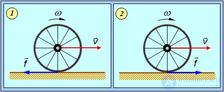
Fig. 7.14. Motion of a hoop with direct spin: 1 –  ; 2 –
; 2 – 
The initial velocity of the lowest point of the hoop is composed of the translational velocity  and the linear velocity
  due to the rotation, directed in the opposite direction. In this connection, two cases must be distinguished.
Case 1 or  . Then the initial velocity
  of the lowest point of the rim is positive, that is, directed in the same direction as the velocity
  . Hence, the friction force f is directed in the opposite direction, as shown in Fig. 11–1. In connection with the change of the positive direction of the rotation axis, it is only necessary to change the sign in front of the second term in equation (7.3.4). The solution of the equations of motion in the case under consideration has the form

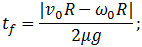
(7.3.14)
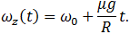
(7.3.15)
With the new choice of direction of the rotation axis, the velocity of the lowest point of the hoop is written in the form

(7.3.16)
The moment  at which slipping disappears is determined from the same relation of the vanishing of the velocity of the lowest point of the hoop, or the equality in magnitude of the oppositely directed velocities of this point due to the translational motion together with the centre of mass and the rotational motion about the axis passing through the centre of mass:
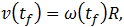
from which we find:
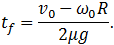
The velocity of the translational motion of the hoop at this moment becomes equal to

and remains unchanged thereafter. This velocity is smaller than the initial velocity of the hoop's translational motion.
Case 2 or  . In this case the velocity of the lowest point of the rim is negative, directed against the velocity
  . Hence, the friction force
  is directed along (see Fig. 11-2).
Correspondingly, in the equations of motion and their solutions (7.3.14) and (7.3.15) the signs in front of the second terms, containing the friction force that has changed direction, must be reversed, and we obtain:

(7.3.17)
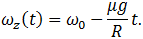
(7.3.18)
Correspondingly, the expression for the velocity of the lowest point of the hoop takes the form:

(7.3.19)
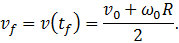
The moment at which slipping ceases  is determined analogously and turns out to be equal to:
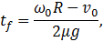
and for the velocity of the steady-state motion we again obtain the expression

but in this case it will be greater () than the initial velocity of the translational motion.
Combining both cases into one, we write the final result:
If a body is set into rotation about an arbitrary axis and then left to itself, the position of the axis of rotation in space will, generally speaking, change: the axis will either turn or shift relative to the inertial frame of reference. In order to keep an arbitrarily chosen axis in a fixed position, certain forces must be applied to it.
An axis of rotation of a body, whose position in space is preserved without the application of any external forces, is called a free axis of the body.
It can be shown that there exist at least three mutually perpendicular axes, passing through the centre of mass of the body, that can serve as free axes. Such axes are called the principal axes of inertia of the body.
The moments of inertia of a body about the principal axes are called the principal moments of inertia.
For bodies possessing axial symmetry (for example, a homogeneous cylinder), one of the principal axes coincides with the axis of symmetry, and any two axes perpendicular to the axis of symmetry and to each other, and passing through the centre of mass of the body, are also principal (Fig. 7.15). The moments of inertia about the latter two axes are equal to each other, while the moment of inertia about the axis of symmetry differs from them

Such a body is called a symmetric top.
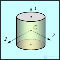
Fig. 7.15. Principal axes of a homogeneous cylinder
For a body with central symmetry (for example, a homogeneous sphere), any three mutually perpendicular axes passing through the centre of symmetry are principal. For them

Such bodies are called spherical tops. Any axis of a spherical top passing through the centre of symmetry is a principal axis (and hence also a free axis).
In the general case the principal moments of inertia of a body are different, that is

Such a body is called an asymmetric top. An example of an asymmetric top can be a homogeneous rectangular parallelepiped (Fig. 7.16).
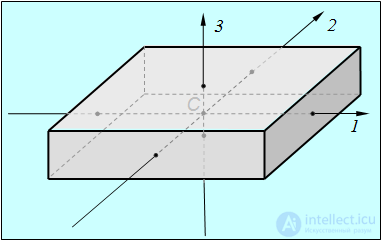
Fig. 7.16. Principal axes of a homogeneous parallelepiped
Under “almost” free rotation, small perturbations may act on the body. If, under such perturbations, the axis of rotation changes its position only slightly, the rotation is called stable. Otherwise one speaks of unstable rotation.
Suppose that for an asymmetric top, for definiteness, the following relation holds between the principal moments of inertia:

It can be shown that rotation about axes 1 and 3 (that is, the axes with the maximum and minimum moments of inertia) will be stable, while rotation about axis 2 (with the intermediate moment of inertia) will be unstable.
Video 7.4. Stability of the flight of a rectangular parallelepiped through the air
Suppose a body rotates about one of the principal axes, for example, about the z axis. Then the angular velocity vector has the form
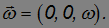
The components of the angular momentum of the body will be equal to

or in vector form

That is, in this case the angular momentum is parallel to the axis of rotation
Video 7.5. Stable rotation of a rod, a disk and a chain about the free axis corresponding to the maximum moment of inertia
If a body rotates in the absence of external forces ( ), then, according to the law of conservation of angular momentum, in this case

In the general case the angular velocity vector rotates about the angular momentum. However, if the axis of rotation coincides with one of the principal axes, the axis of rotation retains its orientation in space in the absence of external forces.
A gyroscope is a massive, axially symmetric body (a symmetric top) rotating rapidly about its axis of symmetry, where the axis of rotation can change its position in space. The axis of symmetry is called the figure axis of the gyroscope.
Video 7.6. What exactly is a gyroscope?
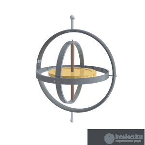
Fig. 7.17. Motion of a system of gyroscopes
The axis of symmetry is one of the principal axes of the gyroscope. Therefore its angular momentum coincides in direction with the axis of rotation.
In order to change the position in space of the axis of the gyroscope's figure, a moment of external forces must be applied to it.
Video 7.7. Gyroscopic forces: a large gyroscope tears a rope
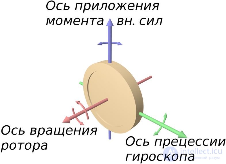
Fig. 7.18. Direction of the vectors during rotation of the gyroscope
In this case a phenomenon is observed that has come to be called gyroscopic: under the action of forces that would seemingly be expected to cause axis 1 to turn about axis 2 (Fig. 7.19), a turning of the figure axis about axis 3 is observed instead.
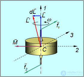
Fig. 7.19. Motion of the gyroscope's figure axis under the action of a moment of external forces
Video 7.8. Gyroscope with weights: direction and speed of precession, nutation
Gyroscopic phenomena occur wherever there are rapidly rotating bodies whose axis can turn in space.
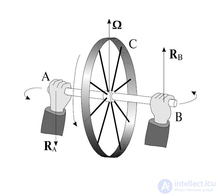
Fig. 7.20. Response of the gyroscope to an external action
The at-first-glance strange behavior of the gyroscope, Fig. 7.19 and 7.20, is fully explained by the equation of the dynamics of rotational motion of a rigid body

Video 7.9. “Amorous” gyroscope: the gyroscope's axis runs along the rail without leaving it
Video 7.10. Action of the moment of friction force: the “Columbus” egg
If the gyroscope is set into rapid rotation, it will possess a considerable angular momentum. If an external force acts on the gyroscope for a time  , the increment of the angular momentum will be
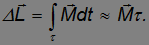
If the force acts for a short time , then
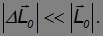
In other words, under short-lived actions (jolts) the angular momentum of the gyroscope practically does not change. This is the source of the gyroscope's remarkable stability with respect to external disturbances, which is used in various instruments such as gyrocompasses, gyro-stabilized platforms, etc.
Video 7.11. Model of a gyrocompass, gyrostabilization
Video 7.12. Large gyrocompass
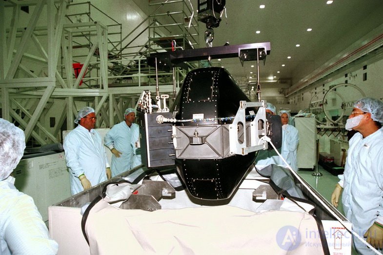
7.21. Gyrostabilizer of an orbital station
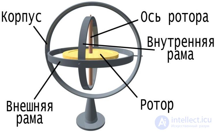
Gyroscopes used in aviation and astronautics employ a gimbal mount, which makes it possible to preserve the direction of the gyroscope's rotation axis regardless of the orientation of the mount itself:
Video 7.13. Gyroscopes in the circus: riding a single wheel along a wire
Let us consider the motion of a gyroscope with a fixed support point, as shown in Fig. 7.22.
The motion of a gyroscope under the action of an external force is called forced precession.
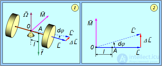
Fig. 7.22. Forced precession of a gyroscope: 1 — general view; 2 — top view
Let us apply at point A a force  . If the gyroscope is not rotating, then, naturally, the right flywheel will descend and the left one will rise. A different situation arises if the gyroscope is first set into rapid rotation. In this case, under the action of the force the gyroscope's axis will rotate with angular velocity
  about the vertical axis. That is, the gyroscope's axis acquires a velocity in the direction perpendicular to the direction of the acting force.
Thus, precession of a gyroscope is a motion under the action of external forces occurring in such a way that the figure axis describes a conical surface.
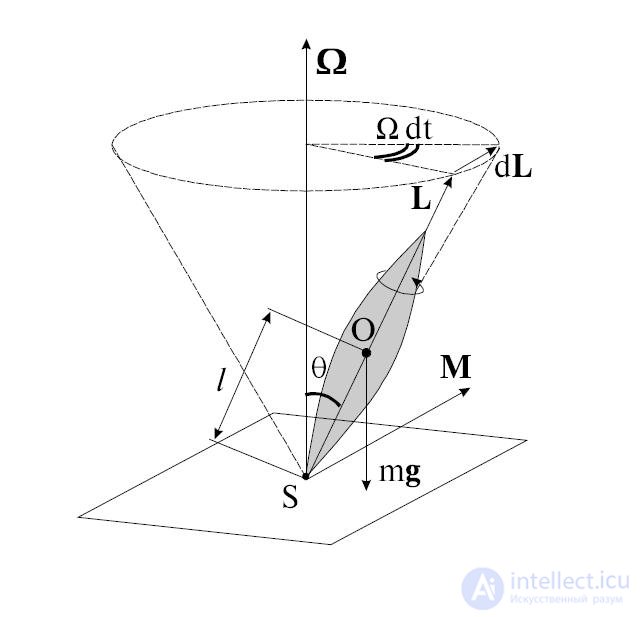
Fig. 7.23. On the derivation of the formula for gyroscope precession.
The explanation of this phenomenon is as follows. The moment of the force about point 0 will be

The increment of the gyroscope's angular momentum over the time  is equal to

This increment is perpendicular to the angular momentum and, consequently, changes its direction, but not its magnitude.
The angular momentum vector behaves in a manner similar to the velocity vector of a particle moving in a circle. In the latter case, the increment of the velocity  is perpendicular to the particle's velocity
  and is equal in magnitude to

where

In the case of a gyroscope, the elementary increment of the angular momentum

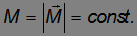
and is equal in magnitude to

moreover
Over the time the angular momentum vector will turn through an angle 
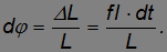
The angular velocity of rotation of the plane passing through the axis of the cone described by the figure axis, and the figure axis itself, is called the angular velocity of precession of the gyroscope.
Oscillations of the gyroscope's figure axis that arise under certain conditions in the plane passing through the axis of the above-mentioned cone and the figure axis itself are called nutations. Nutations can be caused, for example, by a short jolt to the figure axis of the gyroscope upward or downward (see Fig. 7.24):
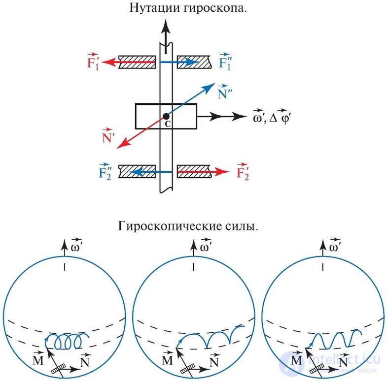
Fig. 7.24. Nutations of a gyroscope
The angular velocity of precession in the case under consideration is equal to
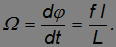
Let us note an important property of the gyroscope — its non-inertness, consisting in the fact that after the external force stops acting, the rotation of the figure axis stops.
The influence of gyroscopic forces in engineering is illustrated by the following figures.
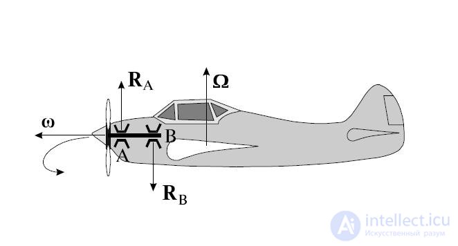
Fig. 7.25. Gyroscopic forces acting on an aircraft as the propeller rotates
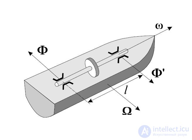
Fig. 7.26. Flipping over of a top under the action of gyroscopic forces
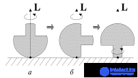
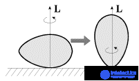
Fig. 7.27. How to stand an egg “on its end”
Appendix
On the principle of operation of the wheel
Since we have talked a great deal in this chapter about the rotation of bodies, let us dwell on the greatest and most important discovery of humankind — the invention of the wheel. Everyone knows that dragging a load is far harder than transporting it on wheels. The question arises, why? The wheel, which plays an enormous role in modern technology, is rightly considered one of the most ingenious inventions of humankind.
Moving a load by means of a roller. The prototype of the wheel was the roller, placed under a load. Its earliest uses are lost in the mists of time. Before we deal with the wheel, let us understand the principle of operation of the roller. For this, let us consider an example.
Example. A load of mass M is placed on a cylindrical roller of mass  and radius
  , which can move along a flat horizontal surface. A horizontal force
  is applied to the load (Fig. 7.28). Let us find the accelerations of the load and the roller. Neglect the rolling friction force. Assume that the motion of the system occurs without slipping.
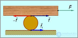
Fig. 7.28. Moving a load by means of a roller
Let us denote by  the friction force between the roller and the load, and by
  — between the roller and the surface. Let us take the direction of the external force as the positive direction. Then positive values of and correspond to the directions of the friction forces shown in Fig. 7.28.
Thus, the forces and act on the load, and the forces and act on the roller. Let us denote by a the acceleration of the load and by a1 — the acceleration of the roller. In addition, the roller rotates clockwise with angular acceleration  .
.
The equations of translational motion take the form:
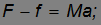

The equation of rotational motion of the roller is written as follows:
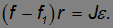
Let us now turn to the conditions of absence of slipping. Because of the rotation of the roller, its lower point has a linear acceleration  and, in addition, participates in translational motion with acceleration
  . In the absence of slipping between the roller and the surface, the total acceleration of the lower point of the roller must equal zero, so that

The upper point of the roller acquires, because of the rotation, an oppositely directed linear acceleration  and the same acceleration of translational motion. For there to be no slipping between the roller and the load, the total acceleration of the upper point must equal the acceleration of the load:

From the equations obtained for the accelerations, it follows that the acceleration of the roller is two times smaller than the acceleration of the load:

and, correspondingly,

From direct experience everyone knows that the roller does indeed lag behind the load.
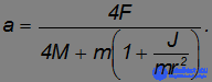
Substituting the relations for the accelerations into the equations of motion and solving them for the unknowns  , , , we obtain the following expression for the acceleration of the load
Both friction forces and turn out in this case to be positive, so that in Fig. 12 their directions were chosen correctly:
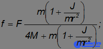
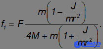
As we can see, the radius of the roller plays no special role: the ratio  depends only on its shape. For a given mass and radius , the moment of inertia of the roller is maximal when the roller is a tube:
  . In this case, the friction force between the roller and the surface is absent ( = 0) and the equations for the acceleration of the load and the friction force between the load and the roller take the form:
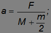
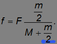
As the mass of the roller decreases, the friction force decreases, and the acceleration of the load increases — the load becomes easier to move.
In the case of a cylindrical roller (a log) /2 and we find the friction forces
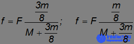
and the acceleration of the load.
Comparing with the results for the tube-roller, we see that the effective mass of the roller has, as it were, decreased: the acceleration of the load increases with other conditions equal.
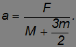
The main conclusion of the example considered: the acceleration is nonzero (that is, the load begins to move) for an arbitrarily small external force. Whereas when dragging a load along a surface, a force of at least  must be applied to shift it.
Second conclusion: the acceleration does not depend at all on the magnitude of the friction between the parts of the given system. The coefficient of friction  does not enter into the solutions found; it appears only in the conditions for absence of slipping, which reduce to the requirement that the applied force must not be too large.
The result obtained, that the roller as it were completely “destroys” the friction force, is not surprising. Indeed, in the absence of relative displacement of the surfaces in contact, friction forces do no work. In fact, the roller “replaces” sliding friction with rolling friction, which we have neglected. In the real case, the minimum force needed to move the system is nonzero, although much smaller than in the case of dragging the load along the surface. In modern technology the operating principle of the roller is realized in ball bearings.
Qualitative examination of the operation of the wheel. Having dealt with the roller, let us move on to the wheel. The first wheel, in the form of a wooden disk mounted on an axle, appears to have arisen in the 4th millennium BC in the civilizations of the Ancient East. In the 2nd millennium BC the construction of the wheel was improved: spokes, a hub and a bent rim appeared. The invention of the wheel gave a colossal boost to the development of crafts and transport. However, many people do not understand the very principle by which the wheel operates. In a number of textbooks and encyclopedias one can find the incorrect assertion that the wheel, like the roller, also gives a gain by replacing sliding friction with rolling friction. Sometimes one hears references to the use of lubrication or bearings, but that is not the point, since the wheel clearly appeared before people thought of lubrication (and, all the more so, bearings).
The action of the wheel is easiest to understand from energy considerations. Ancient carts are constructed simply: the body is attached to a wooden axle of radius (the total mass of the body with the axle equal to M). Wheels of mass and radius R are mounted on the axle (Fig. 7.29).
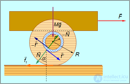
Fig. 7.29. Moving a load by means of a wheel
Suppose that such a cart is being hauled along the same wooden surface (then at all points of contact we have the same coefficient of friction ). First let us jam the wheels and, applying a force , drag the cart a distance s. Since the cart slides along the surface, the friction force reaches its maximum possible value

The work done against this force is equal to

(since the mass of the wheels is usually much less than the mass of the cart <<M).
Let us now free the wheels and again drag the cart the same distance s. If the wheels do not slip on the surface, then at the lower point of the wheel the friction force does no work. But sliding friction arises between the axle and the wheel, at the lower part of the axle of radius . There, too, there is a normal force. It will differ somewhat from the previous one because of the weight of the wheels and other reasons, which we will discuss below, but for a small mass of the wheels and a small coefficient of friction it can be taken as approximately equal to  . Therefore, between the axle and the wheel the same friction force acts

Let us emphasize once again: the wheel by itself does not reduce the friction force. But the work A' done against this force will now be much smaller than in the case of dragging the cart with jammed wheels. Indeed, when the cart travels the distance S, its wheels make  revolutions. This means that the surfaces rubbing against the axle shift relative to each other by a smaller distance
  . Therefore the work done against the friction forces will also be smaller by a corresponding factor:
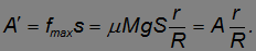
Thus, by putting wheels on axles, we reduce not the friction force, as in the case of the roller, but the path over which it acts. Say, a wheel of radius R = 0.5 m and an axle of radius = 2 cm reduces the work by 96%. The remaining 4% are successfully handled by lubrication and bearings, which reduce the friction itself (lubrication, moreover, prevents wear of the cart's running gear). Now it is clear why such large wheels were made on old carriages and war chariots. Modern supermarket shopping carts can roll at all only thanks to bearings.
From the formula obtained for the work done while rolling it follows that for = R (wheels without an axle, mounted into the body and rubbing against it), the same work would be done as when dragging the cart. The entire gain lies in the ratio of the radii /R, that is, the wheel is, in essence, a continuously acting lever with arms and R. Thanks to the “rolling up” of the lever into a circle, it does not need to be returned to its initial position: this is achieved automatically. It is hard to imagine a technical invention more brilliant in its simplicity and effectiveness!
Quantitative theory of the wheel. Let us consider the forces acting on our cart (see Fig. 7.29).
Forces acting on the wheel: the friction force  from the axle, the normal force
  from the axle, the friction force from the surface. These forces are shown in Fig. 7.29 by blue, green and orange arrows, respectively. Note that we do not assume that the axle touches the wheel at its lowest point: the angle
  describes the backward displacement of the point of contact between the axle and the wheel (correspondingly, the points of application of the forces , ). The value of the angle must also be found from the solutions of the equations of motion. In addition, the force of gravity
  and the normal force
  from the surface act on the wheel, but they are not important to us now and are not shown in the figure.
Choosing the x axis in the horizontal direction and the y axis — in the vertical direction, we write the projection of the equation of translational motion of the wheel onto the x axis:
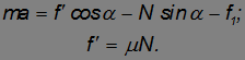
Assuming the absence of slipping at the point of contact of the wheel with the surface (that is  ), we write the equation of rotational motion of the wheel:
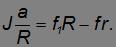
Forces acting on the cart (shown by red, violet, dark blue and dark green arrows, respectively, in Fig. 7.29): the external force  , the force of gravity and the forces
  ,
,  from the axle. Let us write the equations of translational motion of the cart in projections onto the axes x, y:
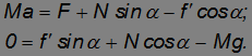
We have five equations for five unknowns:  , , , , . All of them can be found by solving the system of equations. We only want to obtain the answer to the question: at what minimum force
  will the cart move from its place? For this we must set
  , with the acceleration = 0. We then have the system of equations:
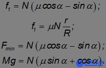
Here we have already taken into account the expression for the law of sliding friction. From the first two equations it follows that:
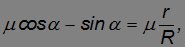
from which the trigonometric functions of the angle can be found:
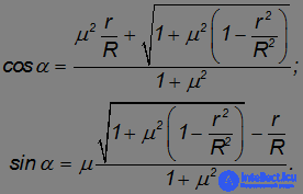
Then from the last two equations follows the desired expression:
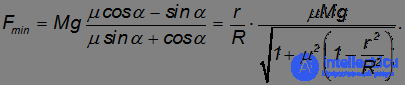
It is curious that the mass of the wheels does not enter into the final answer for  .
.
In the limiting case = R we have  , which corresponds, in essence, to the absence of wheels and the dragging of the cart along the ground. In the opposite limiting case

the minimum force also tends to zero. For small coefficients of friction the square root in the denominator is approximately equal to unity, and
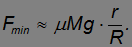
Above we obtained this result qualitatively from energy considerations.


Comments