Spatial self-organization

This series of articles describes a wave model of the brain that is seriously different from traditional models. I strongly recommend that those who have just joined begin reading from the first part.

We proceed from the fact that the phenomena of the external world affect our senses, causing certain signal flows in the nerve cells. In the process of learning, the core acquires the ability to detect certain combinations of signals. The detectors are neurons, the synaptic weights of which are adjusted to the activity patterns corresponding to the detected phenomena. Neurons of the cortex follow their local environment, which forms their local receptive field. Information on the receptive fields of neurons comes either through topographic projection, or through the propagation of waves of identifiers carrying unique patterns corresponding to the already identified features. Detector neurons reacting to the same combination of signs form detector patterns. The patterns of these patterns determine the unique waves of identifiers that these patterns trigger, coming to a state of evoked activity.



In 1952, Alan Turing published a paper entitled “The Chemical Foundations of Morphogenesis” (Turing AM, 1952), devoted to the self-organization of matter. The basic principle formulated by him stated that the global order is determined by local interaction. That is, in order to obtain the structural organization of the entire system, it is not necessary to have a global plan, but you can confine yourself solely to setting the rules for close interaction of the elements forming the system.

Training of neurons does not occur in isolation, but taking into account the activity of their environment. The rules for recording this activity determine the self-organization of the cortex. Self-organization means that in the course of learning not only the detection neuron patterns are formed, but that these patterns are lined up in some spatial structures that have their own specific meaning.

The most obvious way of self-organization is structuring by proximity. It is possible to train neurons in such a way that the patterns corresponding to similar in some sense concepts are close to each other and in the space of the cortex. Later we will see that this placement will be necessary for the implementation of many important functions inherent in the brain. In the meantime, just look at the mechanisms that can provide such an organization.

Quite an ambiguous question - how to measure the closeness of concepts. One approach is connected with the fact that any concept can be compared with a certain description. For example, a description of an event could be a vector, whose components show the severity of certain signs in an event. The set of signs in which the description is kept forms a descriptive basis. In this case, a reasonable measure of closeness is the closeness of descriptions. The closer the description of the two phenomena, the more alike these phenomena are. Depending on the task, which is further solved using the proximity measure, one can choose one or another calculation algorithm. The measure of proximity is closely related to the concept of distance between objects. One can be counted in another and vice versa.

A different approach is the temporary proximity of phenomena. If two phenomena occur simultaneously, but at the same time have different descriptions, then you can still talk about their particular proximity. The more often events occur together, the more their proximity can be interpreted.

In fact, these two approaches do not contradict, but complement each other. If two phenomena often occur together, then it must be concluded that there is a phenomenon that is the realization of this compatibility. This new phenomenon itself may be a sign describing both the original phenomena. Now these phenomena have a common in the description, and therefore, the proximity in the descriptive approach. We will call proximity, which takes into account both descriptive and temporal proximity, as generalized proximity.

Imagine that you are looking at a subject from different angles. Perhaps these species will be completely different in descriptive terms, but nevertheless it is impossible to deny their closeness in some other sense. Temporal proximity is a possible manifestation of this other meaning. Somewhat later, we will develop this topic much deeper, now just note the need to consider both approaches when determining the closeness of concepts.

The simplest to understand neural network, which well illustrates self-organization by the degree of descriptive proximity, is Kohonen's self-organizing maps (figure below).



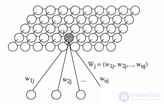
Suppose we have input information given by a vector . There is a two-dimensional lattice of neurons. Each neuron is associated with an input vector. , this relationship is determined by the set of weights wj. Initially, we initiate a network of random small weights. By supplying an input signal, for each neuron one can determine its level of activity as a linear adder. Take the neuron that will show the most activity, and call it the winning neuron. Next, move its weight in the direction of the image, which he was like. Moreover, we will do the same procedure for all its neighbors. We will relax this shift as we move away from the winning neuron.



here - learning rate that falls with time - the amplitude of the topological neighborhood (dependence on n assumes that it also decreases with time).

The amplitude of the neighborhood can be selected, for example, by the Gaussian function:



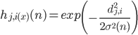
Where - distance between the adjusted neuron and the winning neuron .


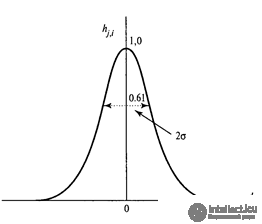Gauss function

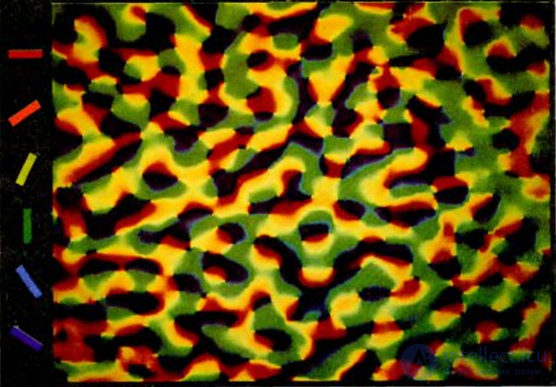
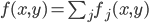
As you learn on such a self-organizing map, zones will be allocated corresponding to how the training images are distributed. That is, the network itself will determine when similar pictures will meet in the input stream, and will create for them close representations on the map. At the same time, the more the images will differ, the more separate their representations will be located apart from each other. As a result, if we appropriately color the learning result, it will look something like the one shown in the figure below.


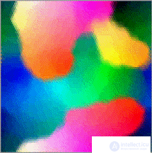The result of learning the card Kohanen

Cohanen maps use the amplitude function of a topological neighborhood, which suggests that neurons, in addition to interacting through synapses, can exchange additional information indicating the nature of the surrounding activity, and this information can influence the course of their synaptic training. The need to transfer additional information arose somewhat earlier in our model. Describing the training of extrasynaptic receptors, we introduced rules based on the knowledge of a certain type of environmental activity by neurons. For example, knowledge of the general level of activity allowed us to make decisions about both the need for training and the rejection of it.

In order to remain in building a model within a certain biological certainty, let us try to show which mechanisms in the real cortex may be responsible for calculating and transmitting additional information that is not encoded into axon signals.

About 40 percent of the brain is occupied by glial cells. Their total number is an order of magnitude greater than the number of neurons. Traditionally, glial cells are assigned a mass of service functions. They create a three-dimensional framework, filling the space between the neurons. Participate in maintaining the homeostasis of the environment. In the process of development of the nervous system involved in the formation of the topology of the brain. Schwann cells and oligodendrocytes are responsible for the myelination of large axons, which leads to a multiple acceleration of the transmission of nerve impulses.

Since glial cells do not generate action potentials, they are not directly involved in information interaction. But this does not mean that they are completely devoid of informational functions. For example, plasma astrocytes are located in the gray matter and have numerous strongly branching processes. These processes encircle the surrounding synapses and affect their work (figure below).


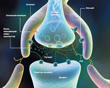Astrocyte and synapse (Fields, 2004)

For example, the following mechanism was described (RD Fields, B. Stevens-Graham, 2002). Activation of a neuron leads to the fact that ATP molecules are released from its axon. ATP (adenosine triphosphate) is a nucleotide that plays an extremely important role in the whole organism, its main function is to provide energy processes. But besides this, ATP can also act as a signal substance. Under its influence, the movement of calcium inside the astrocyte is initiated. This, in turn, leads to the fact that astrocyte releases its own ATP. The result is the transfer of such a state to neighboring astrocytes, which transmit it even further. In this case, the absorption of calcium by astrocytomas leads to the fact that it begins to affect the synapses with which it contacts. Astrocytes can both enhance the synapse reaction by emitting an appropriate mediator, and weaken it due to its absorption or release of neurotransmitter-binding proteins. In addition, astrocytes are able to release signaling molecules that regulate the release of a mediator by the axon. The concept of signal transmission between neurons, taking into account the influence of astrocytes, is called a tripartite synapse.

This interaction of astrocytes and neurons does not transmit specific information images, but it is very well suited to the role of a mechanism that ensures the distribution of the “field of activity”, which can control the training of synapses and thus set the spatial coordinates for the new detector patterns.

In addition to astrocytes, the behavior of synapses is also influenced by the extracellular matrix. A matrix is ​​a multitude of molecules produced by brain cells and filling the extracellular space. The article (Dityatev A., Schachner M., Sonderegger P., 2010) showed that a change in the composition of the matrix affects the nature of synaptic plasticity, that is, the training of neurons.

The impulse activity of neurons creates a point spatial pattern, which dynamically changes, coding information flows. This activity changes the state of the surrounding glial environment and the environment of the matrix in such a way that it creates something like a field of generalized activity (figure below).


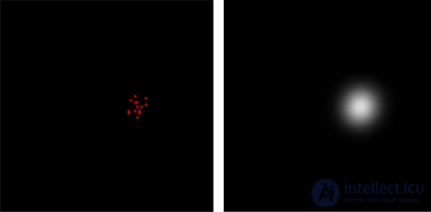Point activity and field of activity

The field of activity, on the one hand, blurs point activity, creating a region that extends beyond the active neurons, on the other hand, has inertia and continues to exist for some time after the cessation of impulse activity.

If inside this field of activity we create a detector of the current supplied image, it will be close to the detectors similar to it. At the same time, similarity may turn out to be both similarity in a receptive field, as well as similarity arising due to combining events over time.

In the real brain, spatial organization is best studied for the zone of the primary visual cortex. Due to the transformations beginning in the retina, a signal arrives at the primary cortex, in which the main information is the lines describing the contours of the objects in the original image. The neurons of the primary visual cortex see mainly small fragments of these lines passing through their receptive fields. It is not surprising that a substantial part of the neurons in this zone are detectors of lines running at different angles.

It was experimentally found that neurons, which are located vertically under each other, respond to the same stimulus. A group of such neurons is called a cortical mini-column. Vernon Mountkasl (V. Mountkasl, J. Edelman, 1981) put forward the hypothesis that for the brain the cortical column is the basic structural unit of information processing.

Earlier, speaking of the patterns of neuron detectors, we depicted them as groups of neurons distributed in a certain local area. This was due to the fact that when modeling, and accordingly, the preparation of pictures used flat neural networks. The real bark is three-dimensional. The bulk of the cortex does not affect our reasoning about the origin and propagation of waves of identifiers. In a three-dimensional crust, waves propagate in the same way as in a flat one. But in the volumetric cortex, nothing prevents us from locating neuron-detectors, forming a single pattern, vertically under each other. This arrangement is neither worse nor better than any others. The main requirement for the pattern is the randomness of its pattern. Since the connections of neurons are randomly distributed, neurons located vertically in one cortical column may well be considered a random pattern. Such a vertical position is quite convenient when determining the place where the detector pattern is created. There is no need to define a local area, but it is enough to indicate the position in which you want to create a pattern. The choice of position may be, for example, where the field of activity is maximal for all free columns of a certain neighborhood. It can be assumed that the cortical minicolon of the real cortex is the detection patterns described in our model.

For traditional models of the cortex, which do not take into account the wave signals, the explanation that all neurons of the mini-column respond to the same stimulus presents a certain difficulty. We have to assume that this is either duplication to ensure resiliency, or an attempt to bring together neurons that respond to one stimulus, but are configured to define it in different positions of the general receptive field. The latter was played up in the neocognitron through the use of simple cell planes. Wave model allows you to look at it from a different angle. It can be assumed that the task of the cortical mini-column is, having recognized a characteristic stimulus, to launch the corresponding wave identifier. Then a few dozen neurons that form a mini-column and react together - this is the mechanism for triggering a wave, that is, the detection pattern.

The organization of orientation columns in the real visual cortex forms the so-called “tops” (“pinwheel”). Such a “top” (figure below (B)) has a center where columns of different orientations converge, and divergent tails, which are characterized by a smooth change in the preferred stimulus. One top forms a hypercolumn. The tails of different hypercolumns transform into each other, forming an orientation map of the cortex (figure below (A)).


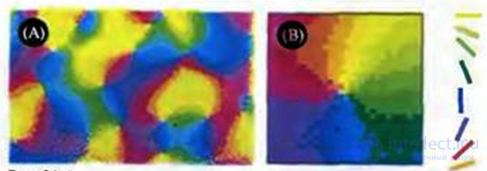Optical distribution of orientation columns in the real crust (J. Nicholls, Martin R., B. Wallace, P. Fuchs, 2003)

Using the example of the visual cortex, it is convenient to compare the actual distribution of orientation columns and the results of modeling using the activity field.

We will feed lines of different angles to a fragment of the cortex. The activity of neuron detectors will be considered as the cosine of the angle between the imaged image and the image on the detector.



Neuron with an index has coordinates on the crust . The value of the field of activity fj from the neuron j at a point with coordinates x, y can be represented, for example, through the Gaussian distribution:



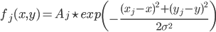
At each point of the cortex, the total value of the activity field can be written down:



We will place new detectors in such a free position, for which the value is maximum. The result of such training is shown in the figure below.


Result of learning of detectors (left), field of activity (right)

As you can see, the simulation result is very similar to the real distribution. But it should be noted that the given example is very conditional. In the real crust, each column is slightly offset relative to its neighbors and follows a slightly different image fragment. This creates “tails” of detectors tuned to one orientation. But at the same time, the stimuli of such detectors are different images, based on different receptive fields.

Spatial self-organization of the crust can be compared with the self-organization of matter in the world around us. Atoms, molecules, objects, planets, stars, galaxies, the universe - all this is a consequence of the existence of four fundamental interactions. It is customary to speak of gravitational, electromagnetic, strong and weak interactions. Particles of matter create around themselves fields corresponding to interactions. Single-type fields are summarized and form the resulting field.The resulting fields affect the particles, determining their behavior. Somewhere the same is true of the brain. It seems that the bark can create several types of fields with different properties. Each of the fields has its effect on the behavior of neurons. The combination of these interactions, for example, can determine the algorithm for learning synapses and thus the spatial organization of neuron-detectors.

It is easy to see that the spatial grouping according to generalized proximity contains an internal contradiction. In this regard, remember the anecdote. Somehow the lion decided to divide the animals into beautiful and intelligent. And here stands the bewildered monkey: "And what am I to do now, burst?" Difficulties arise when the concept being placed turns out to be close to other, distant from each other concepts. For example, if we lay out books on the shelves of the library, then at the same time we want to group them both by genre, and by author, and by original language, and by reader rating. But if the book is only one, then a certain problem arises.

In the process of self-organization of the cortex, it may turn out that the same concept is close in a generalized sense to several others at once, located in different places of the cortex. It does not make sense to place the detector pattern in a compromise way, trying to find some equidistant place. Firstly, there may not be such a place, and secondly, it will completely violate the principle “similar next”. Nothing remains but to create several detector patterns, each in the vicinity of its local maximum field of activity.

At first glance, the duplication of the same concept in different places looks ugly. Working with information, you always want to come to its integration, not spraying. But our model of the neural network allows us to quite elegantly remove the contradictions that have arisen. Each of the detector patterns, although it is created in different places of the cortex, is trained on the same wave of identifiers. Moreover, if we take a two-level construction, one of the levels fixes on itself a fragment of a common identifier wave pattern. This means that the detector patterns scattered in different places are linked together in a single concept with a common identifier.

Such behavior of concepts is a consequence of the previously declared dualism. A concept is both a pattern and a wave. Patterns generate a wave, a wave activates patterns. The spatial position of patterns belonging to one concept characterizes a concept through its proximity to other concepts. The position of the patterns on the cortex, in fact, says a lot about the properties and characteristics of the corresponding phenomenon. But if in Kohonen's maps one area corresponds to one area, as it turns out from the “winner takes all” paradigm, then in our model it is possible not only to give a richer description, but also to preserve the unity of components due to dualism.

Self-organization on the principle of "similar next" is not an end in itself for the cortex. Later we will show that the most important algorithms for the work of the brain require just such an organization and are practically unrealizable outside it.

And now not quite a banal physical analogy. The basic idea of ​​quantum physics is that a quantum system may not be in any possible states, but only in some that are permissible for it. In this case, the quantum system takes no definite value until the measurement takes place. Only as a result of measurement, the system goes into one of the states allowed by it. Under the measurement refers to any external interaction that causes the quantum system to manifest itself.

In quantum physics, a complex-valued function is introduced that describes the pure state of an object, which is called the wave function. In the most common Copenhagen interpretation, this function is related to the probability of finding an object in one of the purest states (the square of the modulus of the wave function is the probability density). A Hamiltonian system is a dynamic system that describes physical processes without dissipation. Until the quantum system interacts, it is Hamiltonian. The behavior of such a system in time and space can be described by describing the evolution of its wave function. This evolution is determined by the Schrödinger equation.



where -Hamiltonian is the operator of the total energy of the system. Its spectrum is the set of possible states in which the system may be after measurement.

When a measurement occurs, the quantum system takes one of the allowed states. This is called the reduction or collapse of the wave function. In the process of measurement, the system ceases to be isolated, and its energy may not be conserved, since energy is exchanged with the device.

What state the quantum system will take at the moment of measurement is a matter of chance. But the probability of choosing each of the states is not the same; it is determined by the value of the wave function associated with this state.

In our model, the detector patterns are created in the positions of the cortex, where the descriptive or temporal proximity of the new concept and concepts of already existing ones is observed. Thus, a set of places is formed that describe the likelihood of a concept in a given situation. This can be compared with the spectrum of the Hamiltonian of the total energy of a quantum system. The propagation of waves of identifiers can be compared with the evolution of the wave function. The description that carries the identifier goes into pattern activity. Further, we will show that this does not activate all patterns, but only those that can describe a consistent picture that corresponds to the context of what is happening. At this moment, our system goes into one of the possible allowed states, which strongly resembles the collapse of the wave function.