Hebba Filter

In the previous section, we described the simplest properties of formal neurons. We talked about the fact that the threshold adder reproduces the nature of a single spike more accurately, and the linear adder allows us to simulate the response of a neuron consisting of a series of pulses. It was shown that the value at the output of the linear adder can be compared with the frequency of the spikes caused by a real neuron. Now we look at the basic properties that such formal neurons possess.

Hebba Filter

Further we will often refer to neural network models. In principle, almost all the basic concepts from the theory of neural networks are directly related to the structure of the real brain. A person, faced with certain tasks, invented many interesting neural network structures. Evolution, going through all possible neural mechanisms, selected everything that turned out to be useful for it. It is not surprising that for very many models, invented by man, you can find clear biological prototypes. Since our narrative does not aim at any detailed description of the theory of neural networks, we will touch only the most general points needed to describe the main ideas. For a deeper understanding, I highly recommend referring to the special literature. For me, the best tutorial on neural networks is Simon Heikin “Neural networks. Full course "(Heikin, 2006).

At the core of many neural network models is the well-known Hebbian learning rule. It was proposed by the physiologist Donald Hebbb in 1949 (Hebb, 1949). In a slightly liberal interpretation, it has a very simple meaning: the connections of neurons that are jointly activated should be strengthened, the connections of neurons that are triggered independently should weaken.
The output state of the linear adder can be written:



If we initiate the initial values ​​of the weights in small quantities and give different images to the input, then nothing prevents us from trying to train this neuron according to Hebb's rule:



where n is a discrete time step, - learning rate parameter.

By this procedure, we increase the weights of those inputs to which the signal is sent. , but we do it all the more, the more active is the reaction of the most trained neuron . If there is no reaction, then there is no learning.

True, such weights will grow indefinitely, so normalization can be applied to stabilize. For example, divide by the length of the vector obtained from the "new" synaptic weights.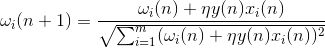



With this training, weights are redistributed between synapses. Understand the essence of redistribution is easier if you follow the changes in weights in two steps. First, when the neuron is active, those synapses that receive a signal receive an additive. Weights of synapses without a signal remain unchanged. Then the total normalization reduces the weights of all synapses. But at the same time, synapses without signals lose in comparison with their previous value, and synapses with signals redistribute among themselves these losses.

Hebb's rule is nothing but the implementation of the gradient descent method on the surface of an error. In fact, we force the neuron to adjust to the signals supplied, each time shifting its weight in the direction opposite to the error, that is, in the direction of the antigradient. In order for the gradient descent to lead us to a local extreme, without skipping over it, the descent speed must be fairly small. That in Hebbovsky training is taken into account by the smallness of the parameter .

The smallness of the learning speed parameter allows you to rewrite the previous formula as a series of :


If we discard the terms of the second order and above, then we get the Oja rule of learning (Oja, 1982):


The positive additive is responsible for Hebbov training, and negative for the overall stability. Writing in this form allows you to feel how such learning can be implemented in an analog environment without using calculations, operating only with positive and negative connections.

So, this extremely simple training has an amazing property. If we gradually reduce the learning rate, then the weights of the synapses of the trained neuron converge to such values ​​that its output begins to correspond to the first main component, which would have been obtained if we applied the corresponding principal component analysis procedures to the supplied data. This design is called a Hebb filter.

For example, we give a pixel image to the input of a neuron, that is, we associate one image point to each neuron synapse. We will feed only two images to the neuron input - images of vertical and horizontal lines passing through the center. One learning step - one image, one line, either horizontal or vertical. If these images are averaged, the cross will be obtained. But the result of training will not be similar to averaging. This will be one of the lines. The one that will be more common in the submitted images. The neuron does not allocate averaging or intersection, but those points that most often occur together. If the images are more complex, the result may not be so clear. But it will always be the main component.

Learning a neuron leads to the fact that a certain image stands out (filtered) on its scales. When a new signal is delivered, the more accurate the signal coincidence and the scale settings, the higher the response of the neuron. A trained neuron can be called a neuron detector. In this case, the image, which is described by its weights, is called the characteristic stimulus.

Main components

The very idea of ​​the principal component method is simple and ingenious. Suppose we have a sequence of events. Each of them we describe through its influence on the sensors with which we perceive the world. Let's say that we have sensors describing signs . All events for us are described by vectors. dimensions . Each component such a vector indicate the value of the corresponding th sign. Together they form a random variable X. These events we can depict as points in -dimensional space, where the signs observed by us will act as axes.



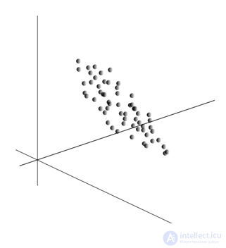
Averaging values gives the mathematical expectation of a random variable X , denoted as E ( X ). If we center the data so that E ( X ) = 0, then the cloud of points will be concentrated around the origin.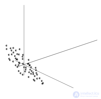



This cloud may be elongated in any direction. Having tried all possible directions, we can find one along which the data dispersion will be maximal.



So, this direction corresponds to the first main component. The main component itself is determined by the unit vector that comes from the origin of the coordinates and coincides with this direction.

Then we can find another direction, perpendicular to the first component, such that along it the dispersion is also the maximum among all perpendicular directions. Finding it, we get the second component. Then we can continue the search by specifying the condition that we should search among the directions perpendicular to the components already found. If the source coordinates were linearly independent, then so we can do times until the dimension of space ends. So we get mutually orthogonal components sorted by the percentage of data variance they explain.

Naturally, the obtained main components reflect the internal laws of our data. But there are more simple characteristics that also describe the essence of the existing laws.

Suppose we have n events in total. Each event is described by a vector. . Components of this vector:


For each feature You can write down how he manifested himself in each of the events:


For any two signs on which the description is based, you can calculate the value showing the degree of their joint manifestation. This value is called the covariance: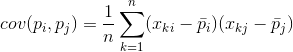


It shows how much the deviations from the mean value of one of the signs coincide in manifestation with similar deviations of another sign. If the mean values ​​of attributes are zero, then the covariance takes the form: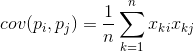


If we correct the covariance by the standard deviations inherent in the signs, then we obtain a linear correlation coefficient, also called the Pearson correlation coefficient:


The correlation coefficient has a remarkable property. It takes values ​​from -1 to 1. Moreover, 1 means the direct proportionality of the two quantities, and -1 means their inverse linear relationship.

Of all the pairwise covariances of attributes, a covariance matrix can be made which, as it is easy to see, is the expectation of the work :


We will further assume that our data are normalized, that is, they have unit variance. In this case, the correlation matrix coincides with the covariance matrix.

So it turns out that for the main components rightly:


That is, the main components, or, as they are called, the factors are eigenvectors of the correlation matrix . They correspond to their own numbers . In this case, the larger the eigenvalue, the greater the percentage of variance explains this factor.

Knowing all the main components for each event which is an implementation of X , you can write its projections onto the main components:


Thus, it is possible to present all the source events in new coordinates, the coordinates of the main components:


In general, there is a distinction between the search procedure for the main components and the procedure for finding the basis of factors and its subsequent rotation, which facilitates the interpretation of factors, but since these procedures are ideologically close and give a similar result, we will call both of them factor analysis.

For a fairly simple procedure of factor analysis lies a very deep meaning. The fact is that if the source feature space is an observable space, then the factors are features that, although they describe the properties of the surrounding world, are generally (if they do not coincide with the observed features) the entities are hidden. That is, the formal procedure of factor analysis allows us to proceed from the phenomena of observables to the discovery of phenomena, although directly and invisible, but nevertheless existing in the surrounding world.

It can be assumed that our brain actively uses the allocation of factors as one of the procedures for cognition of the surrounding world. Selecting factors, we get the opportunity to build new descriptions of what is happening with us. The basis of these new descriptions is the manifestation in the events of those phenomena that correspond to the selected factors.

I will explain a little the essence of the factors at the household level. Suppose you are a personnel manager. Many people come to you, and for each one you fill out a certain form, where you record various observable data about the visitor. After reviewing your notes, you may find that some columns have a certain relationship. For example, a haircut for men will be on average shorter than for women. You are likely to meet bald people only among men, and only women will paint their lips. If factor analysis is applied to personal data, then gender is one of the factors explaining several patterns at once. But factor analysis allows you to find all the factors that explain the correlation dependencies in the data set. This means that in addition to the gender factor, which we can observe, there will be other, including implicit, unobservable factors. And if the floor is explicitly featured in the questionnaire, another important factor will remain between the lines. Assessing the ability of people to express their thoughts, assessing their career success, analyzing their diploma and similar marks, you will come to the conclusion that there is a general assessment of human intelligence, which is not explicitly recorded in the questionnaire, but which explains many of its points. The assessment of intelligence is the hidden factor, the main component with a high explanatory effect. Obviously, we do not observe this component, but we record signs that are correlated with it. Having a life experience, we can subconsciously, according to individual signs, form an idea about the intellect of the interlocutor. That procedure, which our brain uses in this case, is, in fact, a factor analysis. Observing how certain phenomena manifest themselves together, the brain, using a formal procedure, highlights factors as a reflection of the stable statistical patterns inherent in the world around us.

Highlighting a set of factors

We showed how the Hebba filter allocates the first main component. It turns out that using neural networks you can easily get not only the first, but all the other components. This can be done, for example, in the following way. Suppose we have input signs. Take linear neurons where .



Hebb's generalized algorithm (Heikin, 2006)

We will train the first neuron as a Hebb filter, so that it selects the first main component. But each subsequent neuron will be trained on the signal, from which we exclude the influence of all previous components.
The activity of the neurons in step n is defined as


And the amendment to synoptic scales is like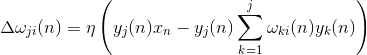

Where from 1 to , but from 1 to .

For all neurons, this looks like learning, similar to Hebb's filter. The only difference is that each subsequent neuron does not see the entire signal, but only that which the previous neurons did not see. This principle is called re-evaluation. We actually, by a limited set of components, restore the original signal and force the next neuron to see only the remainder, the difference between the original signal and the restored one. This algorithm is called the generalized Hebba algorithm.

In the generalized Hebb's algorithm, it is not entirely good that it is too “computational” in nature. Neurons must be ordered, and the calculation of their activities must be strictly sequential. This is not very compatible with the principles of the cerebral cortex, where each neuron, while interacting with the rest, works autonomously and where there is no clearly defined “central processor” that would determine the overall sequence of events. From such considerations, the algorithms, called de-correlation algorithms, look somewhat more attractive.

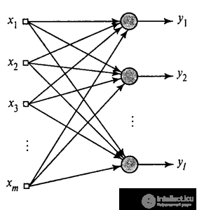
Imagine that we have two layers of neurons Z ₁ and Z ₂ . The activity of the neurons of the first layer forms a certain pattern, which is projected along axons to the next layer.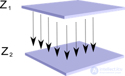


Projection of one layer to another

Now imagine that each neuron of the second layer has synaptic connections with all axons coming from the first layer, if they fall within the boundaries of a certain neighborhood of this neuron (figure below). Axons that fall into such a region form the receptive field of a neuron. The receptive field of a neuron is the fragment of the total activity that is available to it for observation. Everything else for this neuron simply does not exist.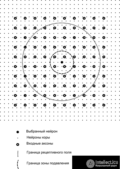



In addition to the receptive field of the neuron, we introduce a region of somewhat smaller size, which we call the suppression zone. Connect each neuron with its neighbors that fall into this zone. Such connections are called lateral or, following the terminology accepted in biology, lateral. We make lateral connections inhibiting, that is, lowering the activity of neurons. The logic of their work - an active neuron inhibits the activity of all those neurons that fall into its zone of inhibition.

Excitatory and inhibitory connections can be distributed strictly with all axons or neurons within the boundaries of the respective areas, and can be set randomly, for example, with a dense filling of a certain center and an exponential decrease in the density of connections as it moves away from it. Сплошное заполнение проще для моделирования, случайное распределение более анатомично с точки зрения организации связей в реальной коре.

Функцию активности нейрона можно записать: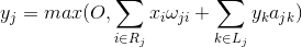

где – итоговая активность, – множество аксонов, попадающих в рецептивную область выбранного нейрона, – множество нейронов, в зону подавления которых попадает выбранный нейрон, – сила соответствующего латерального торможения, принимающая отрицательные значения.

Такая функция активности является рекурсивной, так как активность нейронов оказывается зависимой друг от друга. Это приводит к тому, что практический расчет производится итерационно.

Обучение синаптических весов делается аналогично фильтру Хебба:


Lateral weights are trained according to anti-Hebbovsky rule, increasing inhibition between "similar" neurons:


Суть этой конструкции в том, что Хеббовское обучение должно привести к выделению на весах нейрона значений, соответствующих первому главному фактору, характерному для подаваемых данных. Но нейрон способен обучаться в сторону какого-либо фактора, только если он активен. Когда нейрон начинает выделять фактор и, соответственно, реагировать на него, он начинает блокировать активность нейронов, попадающих в его зону подавления. Если на активацию претендует несколько нейронов, то взаимная конкуренция приводит к тому, что побеждает сильнейший нейрон, угнетая при этом все остальные. Другим нейронам не остается ничего другого, кроме как обучаться в те моменты, когда рядом нет соседей с высокой активностью. Таким образом, происходит декорреляция, то есть каждый нейрон в пределах области, размер которой определяется размером зоны подавления, начинает выделять свой фактор, ортогональный всем остальным. Этот алгоритм называется алгоритмом адаптивного извлечения главных компонент (APEX) (Kung S., Diamantaras KI, 1990).

Идея латерального торможения близка по духу хорошо известному по разным моделям принципу «победитель забирает все», который также позволяет осуществить декорреляцию той области, в которой ищется победитель. Этот принцип используется, например, в неокогнитроне Фукушимы, самоорганизующихся картах Коханена, также этот принцип применяется в обучении широко известной иерархической темпоральной памяти Джеффа Хокинса.

Определить победителя можно простым сравнением активности нейронов. Но такой перебор, легко реализуемый на компьютере, несколько не соответствует аналогиям с реальной корой. Но если задаться целью сделать все на уровне взаимодействия нейронов без привлечения внешних алгоритмов, то того же результата можно добиться, если кроме латерального торможения соседей нейрон будет иметь положительную обратную связь, довозбуждающую его. Такой прием для поиска победителя используется, например, в сетях адаптивного резонанса Гроссберга.

Если идеология нейронной сети это допускает, то использовать правило «победитель забирает все» очень удобно, так как искать максимум активности значительно проще, чем итерационно обсчитывать активности с учетом взаимного торможения.

It's time to finish this part. It turned out for a long time, but I really didn’t want to break up the related narrative. Do not be surprised KDPV, this picture was associated for me at the same time with artificial intelligence and with the main factor.