Perceptron, convolution networks

In the first part, we described the properties of neurons. The second talked about the basic properties associated with their training. Already in the next part we will proceed to the description of how the real brain works. But before that we need to make the last effort and take a little more theory. Now it most likely will seem not especially interesting. Perhaps I myself would have zaminusoval such an educational post. But all this “alphabet” will greatly help us to understand further.

Perceptron

In machine learning, two main approaches are shared: learning with a teacher and learning without a teacher. The previously described methods for isolating the main components are learning without a teacher. The neural network does not receive any explanation for what is given to it at the entrance. It simply highlights the statistical patterns that are present in the input data stream. In contrast, learning with a teacher assumes that for a portion of the input images, called the training sample, we know what output we want to get. Accordingly, the task is to set up a neural network in such a way as to capture the patterns that link the input and output data.

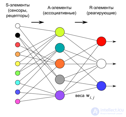
In 1958, Frank Rosenblatt described a design called by him a perceptron (Rosenblatt, 1958), which is capable of learning with a teacher (see KDPV).

According to Rosenblatt, a perceptron consists of three layers of neurons. The first layer is the sensory elements that define what we have at the entrance. The second layer - associative elements. Their connections to the sensory layer are rigidly defined and determine the transition to a more general description than on the sensory layer.

Perceptron training is carried out by changing the weights of the neurons of the third reactive layer. The purpose of training is to force the perceptron to properly classify the submitted images.

The neurons of the third layer work as threshold adders. Accordingly, the weights of each of them determine the parameters of a certain hyperplane. If there are linearly separable input signals, then the output neurons can act as their classifiers.

If a Is the vector of the real output of perceptron a, - the vector that we expect to receive, then the error vector says about the quality of the neural network operation:


If we aim at minimizing the root-mean-square error, then we can derive the so-called delta rule for weighting modification:


In this case, the initial approximation can be zero weights.
This rule is nothing more than the Hebbian rule applied to the perceptron case.
If we place one or more reactive layers behind the output layer and abandon the associative layer, which was introduced by Rosenblatt more for biological certainty than because of computational necessity, then we will get a multilayer perceptron the same as shown in the figure below.


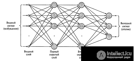Multilayer perceptron with two hidden layers (Heikin, 2006)

If the neurons of the reacting layers were simple linear adders, then there would be little point in such complication. The output, regardless of the number of hidden layers, would still remain a linear combination of input signals. But since threshold adders are used in hidden layers, each such new layer breaks the chain of linearity and can carry its own interesting description.

For a long time it was not clear how a multilayer perceptron can be trained. The main method - the method of back propagation of error was described only in 1974. А.I. Galushkin both independently and simultaneously by Paul J. Verbos. It was then rediscovered and widely known in 1986 (David E. Rumelhart, Geoffrey E. Hinton, Ronald J. Williams, 1986).

The method consists of two passes: direct and reverse. With a direct pass, a training signal is given and the activity of all network nodes, including the activity of the output layer, is calculated. By subtracting the resulting activity from what was required to receive, an error signal is determined. During the back pass, the error signal propagates in the opposite direction, from the output to the input. At the same time, synaptic weights are adjusted in order to minimize this error. A detailed description of the method can be found in a variety of sources (for example, Heikin, 2006).

It is important for us to pay attention to the fact that in a multilayer perceptron information is processed from level to level. In addition, each layer identifies its own set of features characteristic of the input signal. This creates certain analogies with how information is transformed between the areas of the cerebral cortex.

Convolution networks. Neocognitron

Comparison of multilayer perceptron and real brain is very arbitrary. The general is that, rising from zone to zone in the cortex or from layer to layer in the perceptron, the information becomes more and more generalized. However, the structure of the site of the cortex is much more complicated than the organization of the layer of neurons in the perceptron. Studies of the visual system of D. Hubel and T. Wiesel allowed a better understanding of the structure of the visual cortex and prompted the use of this knowledge in neural networks. The main ideas that have been used are the localization of the zones of perception and the division of neurons by functions within one layer.

The locality of perception is already familiar to us, it means that the neuron receiving the information does not follow the entire input space of signals, but only part of it. Earlier we said that this tracking area is called the receptive field of a neuron.

The concept of a receptive field requires separate clarification. Traditionally, the receptive field of a neuron is called the receptor space, which affects the work of the neuron. Receptors here are neurons that directly perceive external signals. Imagine a neural network consisting of two layers, where the first layer is the receptor layer, and the second layer is the neurons connected to the receptors. For each neuron of the second layer, those receptors that have contact with it are its receptive field.

Now take a complex multi-layer network. The further we move away from the input, the more difficult it will be to indicate which receptors and how the neurons in the depth affect the activity. From a certain point, it may turn out that for a neuron all existing receptors may be called its receptive field. In such a situation, only those neurons with which it has direct synaptic contact would be desirable to name the receptive field of a neuron. To separate these concepts, we will call the input receptor space the initial receptive field. And the neuronal space that interacts with the neuron directly - a local receptive field or simply a receptive field, without further clarification.

The division of neurons into functions is associated with the detection of two main types of neurons in the primary visual cortex. Simple (simple) neurons respond to a stimulus located at a specific place in their original receptive field. Complex (complex) neurons are active on the stimulus, regardless of its position.

For example, the figure below shows variants of how the sensitivity pictures of the initial receptive fields of simple cells may look. Positive areas activate such a neuron, negative ones suppress. For each simple neuron there is a stimulus that is most suitable for it and, accordingly, causes maximum activity. But the important thing is that this stimulus is rigidly tied to the position on the initial receptive field. The same stimulus, but shifted to the side, will not cause the reaction of a simple neuron.


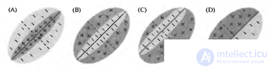The original receptive fields of a simple cell (Nicholls J., Martin R., Wallace B., Fuchs P.)

Complex neurons also have their preferred stimulus, but they are able to recognize this stimulus regardless of its position in the initial receptive field.

From these two ideas, the corresponding neural network models were born. The first such network was created by Kunihik Fukushima. She received the name cognitron. Later he created a more advanced network - neocognitron (Fukushima, 1980). Neocognitron is a multi-layer design. Each layer consists of simple (s) and complex (c) neurons.

The task of a simple neuron is to monitor its receptive field and recognize the image for which it is trained. Simple neurons are collected in groups (planes). Within one group, simple neurons are tuned to the same stimulus, but each neuron watches its fragment of the receptive field. Together, they look through all the possible positions of this image (figure below). All simple neurons of the same plane have the same weight, but different receptive fields. You can imagine the situation in a different way, that this is one neuron that knows how to try on its image at once to all positions of the original image. All this allows you to recognize the same image regardless of its position.


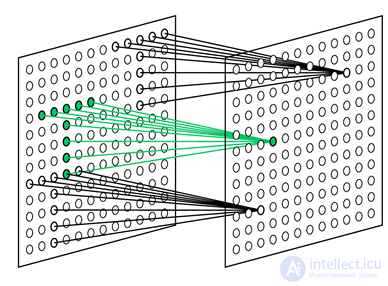Receptive fields of simple cells that are configured to search for a selected pattern in different positions (Fukushima K., 2013)

Each complex neuron monitors its plane of simple neurons and works if at least one of the simple neurons in its plane is active (figure below). The activity of a simple neuron suggests that he recognized a characteristic stimulus in that particular place, which is his receptive field. The activity of a complex neuron means that the same image is encountered on a layer in general, followed by simple neurons.


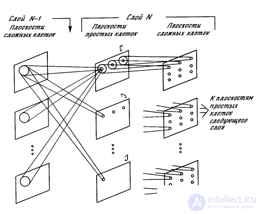Neocognitron Planes

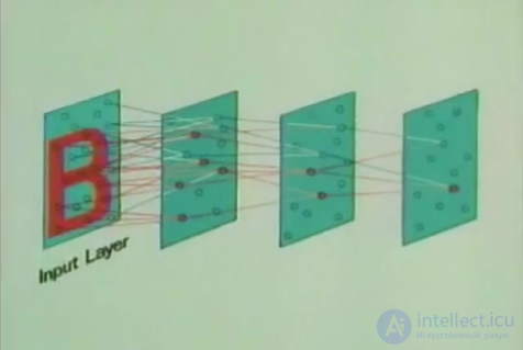
Each layer after the input has its input picture, formed by complex neurons of the previous layer. From layer to layer, an increasing generalization of information occurs, which, as a result, leads to the recognition of specific images regardless of their location in the original image and some transformation.

With regard to image analysis, this means that the first level recognizes lines at a certain angle, passing through small receptive fields. It is able to detect all possible directions anywhere in the image. The next level detects possible combinations of elementary features, defining more complex forms. And so on until such time as it is possible to determine the desired image (figure below).


Neocognitron recognition process

When used for handwriting recognition, such a design is resistant to the way of writing. Recognition success is not affected by movement on the surface or rotation, or deformation (tension or compression).

The most significant difference between a neocognitron and a fully-connected multilayer perceptron is a significantly smaller number of weights used with the same number of neurons. This is due to the “trick” that allows the neocognitron to determine images regardless of their position. The plane of simple cells is essentially one neuron, the weights of which define the core of convolution. This core is applied to the previous layer, running it in all possible positions. Actually, the neurons of each plane and define with their connections the coordinates of these positions. This leads to the fact that all the neurons of the simple cell layer monitor whether the image corresponding to the nucleus appears in their receptive field. That is, if such an image meets anywhere in the input signal for this layer, it will be detected by at least one simple neuron and will cause the activity of the corresponding complex neuron. This trick allows you to find a characteristic image in any place, wherever it appeared. But we must remember that this is precisely a trick and it does not particularly correspond to the work of the real crust.

Neocognitron learning occurs without a teacher. It corresponds to the procedure previously described for isolating a complete set of factors. When real images are fed to the input of the neocognitron, the neurons have no choice but to isolate the components inherent in these images. So, if you give handwritten numbers to the input, then the small receptive fields of simple neurons of the first layer will see lines, angles, and conjugations. The size of the competition zones determines how many different factors can stand out in each spatial region. First of all, the most significant components are distinguished. For handwritten numerals, these will be lines at different angles. If free factors remain, then more complex elements can stand out.

From layer to layer, the general principle of learning is preserved - factors characteristic of a variety of input signals are highlighted. By handing the handwritten numbers to the first layer, at a certain level, we get the factors corresponding to these numbers. Each digit will be a combination of a stable set of features that will stand out as a separate factor. The last layer of the neocognitron contains as many neurons as there are images to be detected. The activity of one of the neurons of this layer indicates recognition of the corresponding image (figure below)


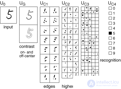Neocognitron Recognition (Fukushima K., Neocognitron, 2007)


An alternative to learning without a teacher is learning with a teacher. So, in the example with figures, we can not wait until the network itself selects statistically stable forms, but tell it what kind of figure it is presented to it, and require appropriate training. The most significant results in such training of convolutional networks were achieved by Yan LeKun (Y. LeCun and Y. Bengio, 1995). He showed how you can use the back-propagation error method to train networks, whose architecture, like that of the neocognitron, remotely resembles the structure of the cerebral cortex.


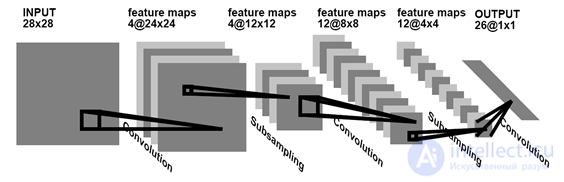Convolution network for handwriting recognition (Y. LeCun and Y. Bengio, 1995)

At this point, we will assume that the minimal initial information is recalled and you can move on to things more interesting and surprising.