
Lecture
Sensitivity analysis (sensitivity analysis) — an assessment of the influence of changes in a project's initial parameters on its final characteristics, for which the internal rate of return or NPV is usually used. The technique of performing sensitivity analysis consists in varying selected parameters within certain limits, on the condition that the remaining parameters stay unchanged. The larger the range of parameter variation over which the NPV or rate of return remains positive, the more stable the project. Sensitivity analysis of a project makes it possible to assess how the project's resulting performance indicators change for different values of the given variables required for the calculation. This type of analysis makes it possible to identify the most critical variables, which can have the greatest effect on the feasibility and effectiveness of the project.
In mathematical modelling, the sensitivity of a response variable (yi) to a parameter (kj) is indicated by the quantity 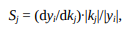 , called the «sensitivity to a parameter» [Ryzhova, 2006: p. 21].
Sensitivity analysis is the study of how the uncertainty in the output of a mathematical model or system (numerical or otherwise) can be divided and allocated to different sources of uncertainty in its inputs. A related practice is uncertainty analysis , which focuses more on quantifying uncertainty and propagating it ; ideally, uncertainty and sensitivity analysis should be carried out together.
Sensitivity analysis of an investment project (sensitivity analysis) – is an assessment of the effect of changes in an investment project's initial parameters (investment costs, cash inflow, discount rate, operating expenses, etc.) on its final characteristics, for which IRR or NPV is usually used.
The sensitivity analysis of a system can be performed, for example, using the fault tree method or the D-factor. .
Sensitivity analysis of a model determines the assessment of the influence of fluctuations in input variable values on the response (output) characteristics of the model . It is necessary to establish over what spread of input data the validity of the main conclusions drawn from the modelling results is preserved.
Sensitivity analysis is understood to mean determining the sensitivity of our final modelling results to changes in the values used for the input variables and model parameters. The analysis determines how the output variable Y changes with small changes in various model parameters or its inputs X.
The ease of performing sensitivity analysis in simulation modelling — is one of the advantages of this method. Sensitivity assessment is an exceptionally important procedure and a preparatory stage before planning a simulation experiment.
The process of recalculating results under alternative assumptions to determine the influence of a variable in sensitivity analysis can be useful for a number of purposes , including:
When studying the sensitivity of models, three types of problems arise [Penenko, 1981, p. 9]:
According to Professor Anthony Atkinson, sensitivity analysis — is the analysis of the effect of a change in a parameter on the solution, rather than on the outcome . The English professor Colin Drury adds: sensitivity analysis assesses how responsive net present value is to changes in the variables used to calculate it .
the relationships between inputs and outputs , may be poorly understood. In such cases the model can be regarded as a black box , i.e. the output is an «opaque» function of its inputs.
Quite often, some or all of a model's input data are subject to sources of uncertainty , including measurement errors , lack of information, and poor or partial understanding of the driving forces and mechanisms. This uncertainty places limits on our confidence in the response or output of the model. In addition, models may have to cope with the natural internal variability of the system (random), such as the occurrence of stochastic events.
Good modelling practice requires that the model developer provide an assessment of the model's reliability. This requires, firstly, a quantitative assessment of the uncertainty of any model results ( uncertainty analysis ); and secondly, an assessment of how much each input contributes to the uncertainty of the output. Sensitivity analysis addresses the second of these questions (although uncertainty analysis is usually a necessary precursor), by ranking the importance, strength and relevance of the input data in determining the variation of the output data.
In models involving many input variables, sensitivity analysis is an important element of model building and quality assurance. National and international agencies involved in impact-assessment research have included sections devoted to sensitivity analysis in their guidelines. Examples are the European Commission (see, for example, its impact assessment guidelines ), the White House Office of Management and Budget , the Intergovernmental Panel on Climate Change and the modelling guidelines of the US Environmental Protection Agency . In a commentary published in 2020 in the journal Nature 22, scientists used COVID-19 as an occasion to propose five ways to make models serve society better. One of the five recommendations, under the heading «Mind the assumptions», is to «perform global uncertainty and sensitivity analysis, [...] allowing everything that is uncertain - variables, mathematical relationships and boundary conditions - to vary simultaneously as the model runs, so that it produces its range of predictions ».
According to Professor Anthony Atkinson, «what if» analysis — is analysis that examines the effect of a change in a parameter on the outcome .
The following are taken as the varied initial variables:
The following may serve as resulting indicators of project performance :
Sensitivity analysis can be carried out in various forms :
The results of sensitivity analysis are presented in tabular or graphical form. The latter is more illustrative and is used for presentation purposes.
When analysing the economic effectiveness of an investment project it is necessary to take into account its uncertainty (incompleteness and inaccuracy of information about the conditions of project implementation), and risk (the possibility of conditions arising that would lead to negative consequences for all or individual participants in the project). Accounting for the uncertainty factor and assessing project risks is provided by sensitivity analysis.
Sensitivity analysis of an investment project (sensitivity analysis) – is an assessment of the effect of changes in an investment project's initial parameters (investment costs, cash inflow, discount rate, operating expenses, etc.) on its final characteristics, for which IRR or NPV is usually used.
Next, the relative change of the criterion relative to the base case is assessed and the sensitivity indicator is calculated. In the course of the sensitivity analysis of an investment project, first the initial parameters (indicators) for which the sensitivity of the investment project is to be calculated are determined. Then a sequential, one-at-a-time change of each selected indicator is carried out. Only one of the variables changes its value by a forecast number of percent (typically 1%, 5% or 10%), and on this basis a new value of the criterion used (for example, NPV or IRR) is recalculated.
The sensitivity indicator is the ratio of the percentage change of the criterion to the change in the value of the variable by the forecast number of percent (the elasticity of the indicator's change). The sensitivity indicators for each of the other selected variables are calculated in the same way.
At the next stage, using the results of the calculations performed, the parameters are ranked by degree of importance (for example, very high, medium and low) and an expert assessment of the predictability (forecastability) of the indicator values is also carried out (high, medium or low).
For sensitivity analysis of an investment project, the main thing – is to assess the degree of influence of a change in each (or a combination) of the initial parameters, in order to anticipate the worst-case development of the situation in the investment project.
Scenario analysis of project development makes it possible to assess the effect on the project of a possible simultaneous change of several variables, through the probability of each scenario. This type of analysis can be carried out either using spreadsheets (for example, Microsoft Excel version 4.0 or higher), or using specialised computer programs that make it possible to use simulation modelling methods.
In the first case, 3—5 project development scenarios are formed. Each scenario should be assigned:
As a result of the calculation, the average values (taking into account the probability of each scenario occurring) of the resulting indicators are determined.
According to international business-planning standards, sensitivity analysis is an integral component of business plans; thus, the United Nations Industrial Development Organization, UNIDO, developed in 1978 the «Guide to Practical Project Appraisal»
The choice of a sensitivity-analysis method is usually dictated by a number of limitations or settings of the problem. Some of the most common are:
Computational cost is an issue for many practical sensitivity analyses. Some methods of reducing computational cost include the use of emulators (for large models) and screening methods (to reduce the dimensionality of the problem). Another method is to use an event-based sensitivity-analysis method to select variables for time-constrained applications. [12] This is the input variable selection (IVS) method, which gathers together tracing information about changes of the system's input and output data using sensitivity analysis to build a matrix of input/output triggers/events, which is designed to map the relationships between input data as causes that trigger events, and output data describing the actual events. The causal relationship between the causes of the state change, i.e. the input variables, and the output parameters of the effects system determines which set of inputs actually affects a given output. The method has a clear advantage over the analytical and computational IVS method, since it attempts to understand and interpret the change of the system's state in the shortest possible time with minimal computational cost. [12] [13]
In uncertainty and sensitivity analysis there is a crucial trade-off between how scrupulously the analyst examines the initial assumptions and how broad the resulting conclusions can be . This is well illustrated by the econometrician Edward E. Leamer : [16] [17]
I have proposed a form of organised sensitivity analysis, which I call «global sensitivity analysis», in which a range of alternative assumptions is chosen and the corresponding interval of conclusions is determined. Conclusions are considered reliable only if the domain of assumptions is wide enough to inspire confidence, and the corresponding interval of conclusions is narrow enough to be useful.
Note. Leamer places emphasis on the need for «credibility» when choosing assumptions. The simplest way to invalidate a model is to demonstrate that it is fragile with respect to uncertainty in the assumptions, or to show that its assumptions were not accepted «widely enough». The same concept is expressed by Jerome R. Ravetz, for whom bad modelling is when the uncertainties of the input data must be suppressed so that the output data does not become uncertain.
Some common difficulties in sensitivity analysis include:
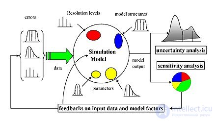
An idealised sensitivity analysis scheme, possibly sample-based. Uncertainty arising from various sources - errors in the data, parameter estimation procedures, alternative model structures - is propagated through the model for uncertainty analysis, and its relative importance is quantified by means of sensitivity analysis.
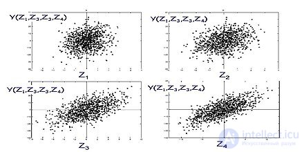
Sample-based sensitivity analysis using scatter plots. Y (the vertical axis) is a function of four factors. The points on the four scatter plots are always the same, although sorted differently, that is, by Z 1 , Z 2 , Z 3 , Z 4 in turn. Note that the abscissa is different for each plot: (-5, +5) for Z 1 , (-8, +8) for Z 2 , (-10, +10) for Z 3 and Z 4 . Z 4 is the most important in influencing Y , as it gives more «shape» to Y .
There are many approaches to performing sensitivity analysis, many of which were developed to address one or more of the limitations described above. They also differ in the type of sensitivity measure, whether based on (for example) variance decomposition, partial derivatives, or elementary effects. However, in general, most procedures adhere to the following scheme:
In some cases this procedure will be repeated, for example in high-dimensional problems where the user must screen out unimportant variables before performing a full sensitivity analysis.
The various types of «core methods» (discussed below) differ in the various sensitivity measures they calculate. These categories may overlap in some way. Alternative ways of obtaining these measures may be proposed given the constraints of the problem.
One of the simplest and most common approaches is to change one factor at a time (OAT) to see what effect this has on the outcome. [23] [24] [25] OAT typically involves
Sensitivity can then be measured by tracking the changes in the output, for example using partial derivatives or linear regression. This seems a logical approach, since any change observed in the output will unambiguously be attributable to the change of a single variable. Moreover, by changing one variable at a time, all other variables can be kept fixed at their central or baseline values. This increases the comparability of the results (all «effects» are calculated relative to the same central point in space) and minimises the likelihood of computer program failures, which is more likely when several input factors are changed simultaneously. Modellers often prefer OAT for practical reasons. In the event of a model failure during OAT analysis, the model developer immediately knows which input factor is causing the failure. [14]
However, despite its simplicity, this approach does not fully explore the input space, since it does not take into account simultaneous changes in the input variables. This means that the OAT approach cannot detect the presence of interactions between input variables. [26]
Methods based on the local derivative involve taking the partial derivative of the output Y with respect to the input factor X i :

where the subscript X 0 indicates that the derivative is taken at some fixed point in the input space (hence «local» in the class name). Adjoint modelling [27] [28] and automatic differentiation [29] are methods of this class. Like OAT, local methods do not attempt to fully explore the input space, since they explore small perturbations, usually one variable at a time.
Regression analysis in the context of sensitivity analysis involves fitting a linear regression to the model response and using standardised regression coefficients as direct sensitivity measures. The regression must be linear with respect to the data (i.e. a hyperplane, hence no quadratic terms, etc. as regressors), because otherwise it is difficult to interpret the standardised coefficients. Therefore this method is most suitable when the model response is in fact linear; linearity can be confirmed, for example, if the coefficient of determination is large. The advantages of regression analysis are that it is simple and has low computational cost.
Variance-based methods [30] [31] [32] are a class of probabilistic approaches that quantitatively define input and output uncertainties as probability distributions and decompose the output variance into parts attributable to input variables and combinations of variables. Thus, the sensitivity of the output to an input variable is measured by the amount of output deviation caused by that input. They can be expressed as conditional expectations, i.e., considering the model Y = f ( X ) for X = { X 1 , X 2 , ... X k }, the sensitivity measure of thei-th variable X i is given as,

where «Var» and « E » denote the variance and expected value operators respectively, and X ~ i denotes the set of all input variables except X i . This expression essentially measures only the contribution of X i to the uncertainty (variance) of Y (averaged over the variations of the other variables) and is known as the first-order sensitivity index or main effect index . It is important to note that it does not measure the uncertainty caused by interaction with other variables. Another measure, known as the total effect index , gives the total variance of Y, caused by X i. and its interactions with any other input variables. Both quantities are usually standardised by dividing by Var ( Y ).
Variance-based methods allow the input space to be fully explored, taking into account interactions and nonlinear responses. For these reasons, they are widely used when they can be calculated. This calculation typically involves the use of Monte Carlo methods, but since it may involve many thousands of model runs, other methods (e.g. emulators) can be used where necessary to reduce computational cost. Note that full variance decomposition is only meaningful if the input factors are independent of each other. [33]
One of the main shortcomings of the previous sensitivity analysis methods is that none of them take into account the spatially ordered structure of the response surface / model output data Y = f ( X ) in the parameter space. Using the concepts of directional variograms and covariograms, variogram analysis of response surfaces (VARS) addresses this shortcoming by recognising the spatially continuous correlation structure for the values of Y , and consequently for the values of .
.
Essentially, the higher the variability, the more heterogeneous the response surface is along a given direction/parameter at a given perturbation scale. Accordingly, within VARS, the values of directional variograms for a given perturbation scale can be regarded as a comprehensive illustration of sensitivity information, linking variogram analysis to the concepts of both the direction and scale of perturbation. As a result, the VARS framework accounts for the fact that sensitivity is scale-dependent, and thus overcomes the scaling problem of traditional sensitivity analysis methods. [36]More importantly, VARS can provide relatively stable and statistically robust estimates of parameter sensitivity at a much lower computational cost than other strategies (approximately two orders of magnitude more efficient). [37] Notably, it has been shown that there is a theoretical relationship between the VARS framework and variance- and derivative-based approaches.
Screening is a special case of the sample-based method. The task here is rather to determine which input variables make a significant contribution to the uncertainty of the output data in high-dimensional models, rather than precisely quantifying sensitivity (i.e. in terms of variance). Screening generally has a relatively low computational cost compared to other approaches, and can be used in preliminary analysis to screen out non-influential variables before applying more informative analysis to the remaining set. One of the most commonly used screening methods is the elementary effects method . [38] [39]
A simple but useful tool is to plot scatter graphs of the output variable against individual input variables after (random) sampling of the model over the input distributions. The advantage of this approach is that it can also work with «given data», i.e. a set of arbitrarily placed data points, and gives a direct visual indication of sensitivity. Quantitative measures can also be obtained, for example by measuring the correlation between Y and X i or even by estimating variance-based measures using nonlinear regression . [15]
A number of methods have been developed to overcome some of the limitations discussed above, which would otherwise make it impossible to estimate sensitivity measures (most often due to computational cost). As a rule, these methods are focused on the efficient calculation of variance-based sensitivity measures.
Emulators (also known as metamodels, surrogate models, or response surfaces) are data-modelling/machine-learning approaches that involve constructing a relatively simple mathematical function, known as an emulator , that approximates the input/output behaviour of the model itself. [40] In other words, this is the concept of «modelling the model» (hence the name «metamodel»). The idea is that, although computer models may represent a very complex series of equations that may take a long time to solve, they can always be treated as a function of their input data Y = f ( X). By running the model at several points in the input space, a much simpler emulator η ( X ) can be fitted, such that η ( X ) ≈ f ( X ) to within an acceptable margin of error. [41] Sensitivity measures can then be calculated using the emulator (via Monte Carlo or analytically), which will require negligible additional computational cost. It is important to note that the number of model runs needed to fit the emulator can be orders of magnitude smaller than the number of runs required for a direct estimation of sensitivity measures from the model. [42]
It is clear that the essence of the emulator approach is to find η (the emulator) that is a sufficiently close approximation to the model f . This requires the following steps,
Sampling of the model can often be done using low-discrepancy sequences, such as the Sobol sequence - named after the mathematician Ilya M. Sobol - or Latin hypercube sampling, although random designs can also be used with some loss of efficiency. The choice of emulator type and training are inherently linked, since the training method will depend on the class of emulator. Some types of emulators that have been successfully used for sensitivity analysis include:
Using an emulator poses a machine learning problem, which can be difficult if the model response is highly nonlinear . In all cases, it is useful to check the accuracy of the emulator, for example using cross-validation .
High-dimensional model representation (HDMR) [47] [48] (a term attributed to H. Rabitz [49]) is essentially an emulator approach that involves decomposing the function's output data into a linear combination of input terms and interactions of increasing dimensionality. The HDMR approach exploits the fact that a model can usually be well approximated by neglecting higher-order interactions (second- or third-order and above). Each term of the truncated series can then be approximated, for example by polynomials or splines (REFS), and the response expressed as a sum of main effects and interactions up to the truncation order. From this point of view, HDMR can be regarded as emulators that neglect high-order interactions; the advantage is that they can emulate higher-dimensional models than full-order emulators.
High-dimensional model representation is a finite expansion for a given function of many variables . The expansion was first described by Sobol as

The technique for determining the right-hand-side functions is given in Sobol's paper. A review can be found here: High Dimensional Model Representation (HDMR): concepts and applications .
The Fourier Amplitude Sensitivity Test (FAST) uses a Fourier series to represent a multidimensional function (model) in the frequency domain using a single frequency variable. Consequently, the integrals required to calculate the sensitivity indices become one-dimensional, resulting in computational savings.
Methods based on Monte Carlo filtering. [50] [51] They are also sample-based, and here the goal is to identify regions in the space of input factors that correspond to particular values (e.g. high or low) of the output data.
The purpose of sensitivity analysis – is to determine the degree of influence that a change in the model's (project's) source data has on the final result (profitability, income, payback period - any chosen indicator). Sensitivity analysis consists in determining the critical boundaries of change of factors. For example, by how much can sales volumes or prices for products, works, or services be reduced at most while the net present value (NPV) remains positive. The wider the range of parameters within which performance indicators remain within acceptable values, the higher the project's margin of safety, the better it is protected against fluctuations in the various factors that influence the results of the project's implementation. The algorithm for performing sensitivity analysis:
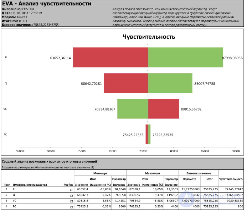
Sensitivity analysis. Calculation results on an Excel sheet
The calculations and the chart show exactly which change in the input parameters the project can withstand.
Sensitivity analysis has limitations :
Examples of sensitivity analysis can be found in various fields of application, such as:
It may happen that the sensitivity analysis of a model-based study is intended to reinforce a conclusion and confirm its reliability in a context where the conclusion is taken into account in policy or decision-making. In these cases, the framing of the analysis itself, its institutional context, and the motivation of its author may become a matter of great importance, and a pure sensitivity analysis - with its emphasis on parametric uncertainty - may be considered insufficient. The emphasis on framing may be due, among other things, to the relevance of the policy study to various interest groups, which are characterised by different norms and values, and hence a different narrative about «what the problem is» and, above all, about «who is telling the tale'. Most often, the frame includes more or less implicit assumptions,
In order to properly address these issues, SA tools have been extended to provide an assessment of the entire process of knowledge and model creation. This approach has been called «sensitivity auditing». It is based on NUSAP [52], a method used to determine the value of quantitative information by creating "pedigrees" of numbers. Similarly, sensitivity auditing has been developed to obtain pedigrees of models and model-based conclusions. [53] Sensitivity auditing was specifically designed for an adversarial context, where not only the nature of the evidence but also the degree of certainty and uncertainty associated with the evidence will be the subject of partisan interests. [54]Sensitivity auditing is recommended in the European Commission's impact assessment guidelines, as well as in the «Scientific Advice for Policy» report of the European Academies. [55]
Sensitivity analysis is closely related to uncertainty analysis; while the latter studies the overall uncertainty in the conclusions of a study, sensitivity analysis attempts to determine which source of uncertainty has a greater influence on the study's conclusions.
The formulation of the problem in sensitivity analysis also has a great deal in common with the field of design of experiments . [56] In design of experiments, the effect of some process or intervention («treatment») on some objects («experimental units») is studied. In sensitivity analysis, the effect of changing the input data of a mathematical model on the model's own output data is considered. In both disciplines, the aim is to obtain information from a system with a minimum of physical or numerical experiments.

Comments