
Lecture
Structure of an electrical circuit. An electrical circuit consists of devices, whose contacts are connected to one another at points called nodes. We shall consider two-contact devices. Electric current flows from node to node through a device. The state of the electric current at any moment of time is characterised by its magnitude (strength), and the state of a node is characterised by its potential.
Current strength. The strength of a direct current equals the charge passing through the cross-section of a device per unit time. In the general case, the current strength and the charge are related by an integral relation:
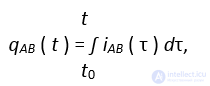
where qAB ( t ) - is the charge that passed through the device from node A to node B from the moment of time t0, when the current was switched on, up to the moment of time t, and iAB ( τ ) - is the current strength flowing through the device at the moment of time τ. If the function iAB ( τ ) is continuous, then iAB ( t ) = q'AB ( t ).
Kirchhoff's first rule. Kirchhoff's first rule is a consequence of the law of conservation of charge: the sum of the currents flowing into a node equals the sum of the currents flowing out of the node.
The potential of a node. The potential of a node equals the work that must be expended, in overcoming electrostatic forces, to move a unit positive charge from a fixed point to the given node. In electrical engineering, a point on the surface of the Earth is chosen as the fixed point, so that the potential of the Earth's surface is equal to zero. From the law of conservation of energy it follows that a unit positive charge moving along an electrical circuit from node A to node B acquires energy equal to the difference of their potentials φA - φB.
The generalised Ohm's law. The generalised Ohm's law states that the magnitude of the change in energy of a unit positive charge passing through a device is proportional to the current strength:
the voltage drop across a device connecting nodes A and B is computed by the formula:
UAB = iAB R = φA - φB + eAB
where iAB – is the current flowing through the device from node A to node B ( iAB = - iBA), R – is the resistance of the device, φA – is the potential of node A, φB - is the potential of node B, eAB – is the electromotive force of the device, eAB = - eBA . If the device contains a source of electromotive force, then the magnitude of this source is considered positive in the case when the current passes through the device from the node with lower potential to the node with higher potential.
An electrical circuit consisting of a source of constant electromotive force and a resistance. Consider an electrical circuit consisting of a source of constant electromotive force (EMF) and a resistance, where the positive pole of the EMF source is connected to a contact of the resistance at node A, and the negative pole of the EMF source is connected to the other contact of the resistance at node B. From Kirchhoff's first rule it follows that at every moment of time the current strength flowing from node A to node B through the resistance equals the current strength flowing from node B to node A through the EMF source. Let us denote this current strength by the symbol i. Applying the generalised Ohm's law to the EMF source, we obtain:
iAB ∙ 0 = φB - φA + eBA
(the EMF source is ideal — its resistance equals zero),
eBA = φA - φB.
On the other hand,
i R = φA — φB,
where R — is the value of the resistance. Thus,
i = eBA / R
Kirchhoff's second rule. Let us write the generalised Ohm's law for each device belonging to a closed loop of the electrical circuit and add the resulting equalities. The sum of the potentials of all nodes of the loop reduces to zero, so that the sum of the voltage drops around the closed loop equals the sum of the electromotive forces of the devices forming that loop (Kirchhoff's second rule).
The electromotive force of a coil. The electromotive force of a coil (without a core) is computed by the formula
eAB ( t ) = - L ( iAB ( t ))',
where L – is the self-inductance coefficient of the coil.
An electrical circuit consisting of a source of constant electromotive force, a coil and a resistance. The electrical circuit consists of a switch, a source of constant electromotive force of magnitude e0, resistance and a coreless coil; the resistance value equals R, the coil's self-inductance coefficient equals L (one must distinguish the cases where the letter L denotes the coil's self-inductance coefficient and where it denotes the Laplace transform). We consider an ideal electrical circuit — the source of electromotive force and the coil have no internal resistance. At the initial instant of time t = 0 the electric current is switched on. From Kirchhoff's first law it follows that the current strengths flowing through the devices making up the electrical circuit are equal; let us denote the strength of each of these currents at time t by i ( t ) Applying Kirchhoff's second law, we obtain the equation
R i ( t ) = χ ( t ) e0 - L i' ( t ).
At the initial instant of time t = 0 there is no current in the circuit: i ( 0 + 0 ) = 0 — this is the initial condition of our problem.
Electromotive force of the capacitor. The charge accumulated by the capacitor is proportional to its electromotive force:
qAB ( t ) = - C eAB ( t ),
the coefficient C is called the electrical capacitance of the capacitor.
An electrical circuit consisting of a constant electromotive force source, a capacitor and a resistance. The electrical circuit consists of a switch, a source of constant electromotive force of magnitude e0, a resistance and a capacitor; R – the resistance value, C — the capacitance of the capacitor. At the initial instant of time t = 0 the electric current is switched on. From Kirchhoff's first law it follows that the current strengths flowing through the devices making up the electrical circuit are equal; let us denote the strength of each of these currents at time t by i ( t ) Applying Kirchhoff's second law, we obtain the equation
R i ( t ) = χ ( t ) e0 - q ( t ) / C.
At the initial instant of time t = 0 the charge of the capacitor equals zero: q ( 0 + 0 ) = 0 — this is the initial condition of our problem.
We take the state of the system to be described by the value of the capacitor charge q ( t ), while the current is a continuous function of time. Since
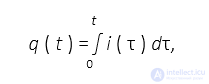
then the current is the derivative of the charge: q' ( t ) = i ( t ),
R q' ( t ) + q ( t ) / C = χ ( t ) e0.
One of the most widespread methods for forming and implementing mathematical models of electrical circuits is the state-variable method. Its application involves dividing all the variables relating to the electrical circuit diagram into three sets:
The input variables are taken to be the driving voltages e(t) of ideal voltage sources and the driving currents j(t) of ideal current sources; the state variables are the currents in the inductances iL(t) and the voltages across the capacitances UC(t), while the output variables are all the remaining currents and voltages that need to be determined in the calculation.
The mathematical model of an electrical circuit in the state-variable method is formed as a system of first-order differential equations written in normal form (Cauchy form):
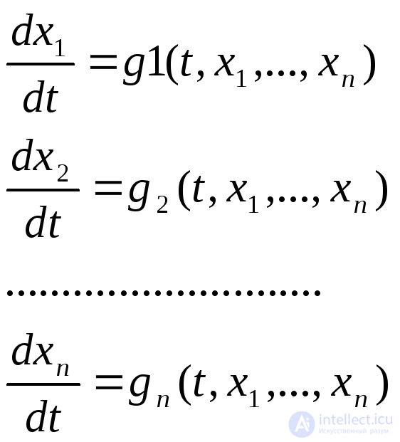 (2.7)
(2.7)
It is convenient to represent the system of differential equations (2.7) in matrix form:
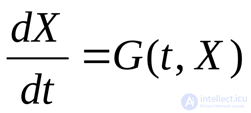 (2.8)
(2.8)
where X= [x1,x2,…,xn]T– is the single-column matrix (vector) of state variables;G(t,X) = [g1(t,X),g2(t,X),…,gn(t,X)]T–n-dimensional vector function.
When it is necessary to determine the output variables, the system of differential equations is supplemented by a system of algebraic equations relating the output variables to the input variables and to the state variables:
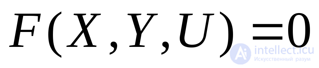 (2.9)
(2.9)
where Y= [y1,y2,…,yk]T- vector of output variables;
F(X,Y,U) = [f1(X,Y,U),f2(X,Y,U),…,fk(X,Y,U)]T–k-dimensional vector function.
For a linear electrical circuit with constant parameters, the mathematical model is a system of linear inhomogeneous differential equations, as well as linear algebraic equations with constant coefficients:
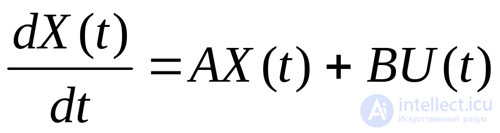
 (2.10)
where A,B,C,D -matrices of constant coefficients of the equations, andA -is a square matrix of order n(n -the number of state variables),B-a matrix of size n x p{p -the number of input variables),C –a matrix of size kxn (k -the number of output variables),D -a matrix of size kxp.
The basis for forming mathematical models of electrical circuits containing two-terminal elements with constant parameters is Kirchhoff's first and second laws and the component relations (2.1, 2.2) for resistive, inductive and capacitive elements.
Here, at the first stage, a system of equations is compiled:
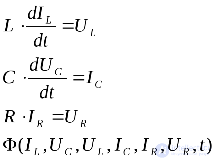 (2.11)
Here IL,IR,IC– are the single-column matrices of the currents in the inductances, resistances and capacitances respectively;UL,UR,UC– are the single-column matrices of the voltage drops across the inductances, resistances, capacitances;L,C,R -diagonal matrices of the inductances, capacitances, resistances;F -a single-column matrix whose elements are functions of the indicated variables. The first two matrix equations constitute a system of differential equations with respect to the state variables, while the last two constitute a system of algebraic equations relating the state variables to the remaining variables.
At the second stage of forming the mathematical model, the system of equations (2.11) is transformed into a system consisting only of differential equations with respect to the state variables and the input variables. To do this, the variables ULand ICare expressed from the system of algebraic equations in terms of the state variables and the input variables and substituted into the right-hand sides of the differential equations from (2.11). However, complications may arise here due to incompleteness of the system of algebraic equations. If the system of algebraic equations in (2.11) is complete, that is, the number of variablesUL,IC,IR,URequals the number of equations and the system is solvable with respect to the indicated variables, then transforming the model into a system consisting only of differential equations is possible, and the order of the system of differential equations will equal the number of reactive elements in the circuit. If, however, the system of algebraic equations is incomplete, transformation into a system consisting only of differential equations is still possible, but the order of the system of differential equations will be lower than the number of reactive elements in the circuit. Such circuits are called topologically degenerate. Topologically degenerate electrical circuits include circuits containing loops made up of capacitances and ideal voltage sources, as well as circuits containing stars made up of inductances and ideal current sources.
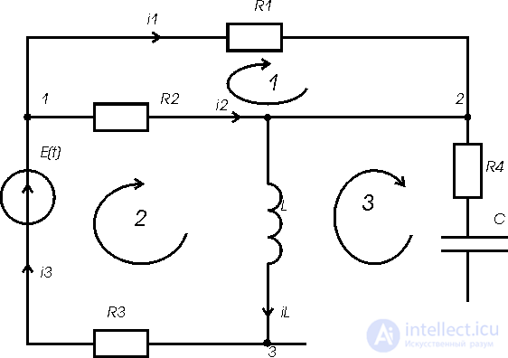
Diagram of the electrical circuit, fig. 3.1


number of nodes Nnode = 3
number of branches Nbr =5
number of branches containing only an ideal EMF source = 0
number of branches containing only an ideal current source = 0
In accordance with ( ), by Kirchhoff's first law it is necessary to compile 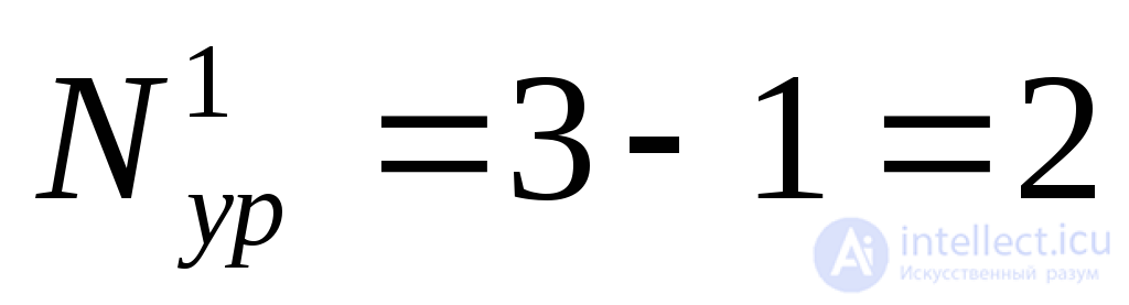

the required number of equations by Kirchhoff's second law 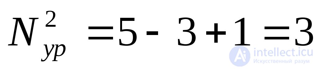
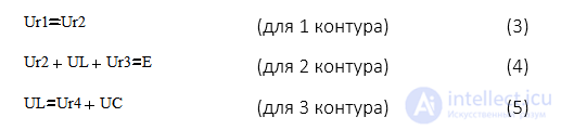
Component relations for the circuit:

Substituting Ur4 into equation (5), we obtain:

From equation (2) we express iC and substitute it into equation (6):

We express the current i3 from equation (4):

Equating equations (8) and (1)

Substituting Ur2, we obtain:

From equation (3) we express i1:

We substitute equation (11) into equation (10):

From equation (12) we find i2

We substitute equation (11) into equation (7)

We substitute equation (14) into equation (13):

We express UL:

Simplifying, we obtain:

Taking into account the relation:  we obtain:

Then:

From equation (5)

We substitute equation (17) into equation (18)

Let us group the data:

Taking into account the relation  we obtain:

Then

We express the specified output variable Ur3 from equation (4)

Taking into account the relation  , we obtain:

Substituting i2 from equation (13)

We substitute UL

The mathematical model is a system of two first-order differential equations with constant coefficients:

Let us represent the system of equations in matrix form:
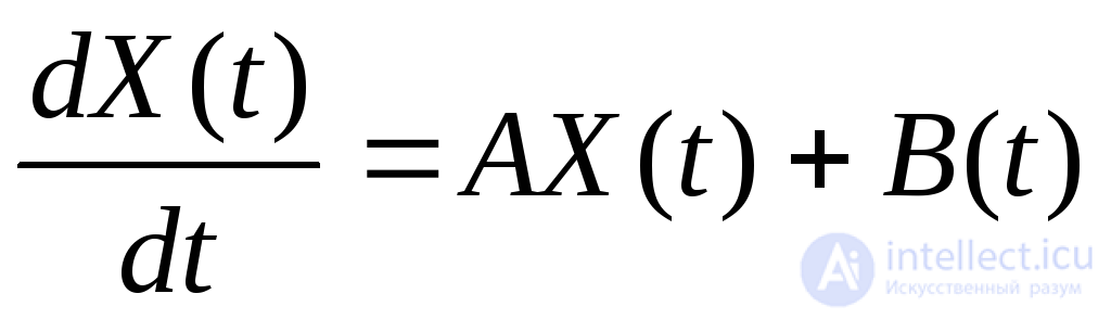 ,
,
or, taking into account the nature of the driving voltage:
 ,
,
where  - is the vector of state variables;

- is a second-order square matrix of constant coefficients of the state variables in the model equations.

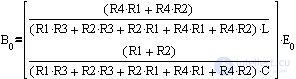 ;
;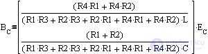
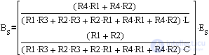
- are the vectors of external action.
The expression for determining the specified output variable in terms of the state variables has the form:
From equation (4) we find Ur3

Using the relation,  we rewrite equation (23)
 (24)
(24)
We substitute the value of current I2 from equation (13)
 (25)
(25)
We substitute the value of UL from equation (17)
 (26)
(26)
We obtain:

Optimal point
p =0.000100
p =0.006125
kpmax=0.642507
Eigenvalues:
l =-1.63277670438401E+0000
l =:-1.47074460251033E+0004
Time constants:
taul= 6.12453618008510E-0001
tau2= 6.79927703486489E-0005
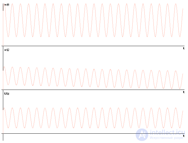
Transient process

Comments