
Lecture
Petri nets - a mathematical apparatus for modelling dynamic discrete systems. They were described in the doctoral dissertation of Carl Petri, "Kommunikation mit Automaten," submitted for the degree of Doctor of Science in 1962. A Petri net is a bipartite directed graph consisting of vertices of two types - places and transitions - connected to one another by arcs. Vertices of the same type cannot be connected directly. Places may hold tokens (markers), which are able to move around the net.

Petri nets - a modelling tool
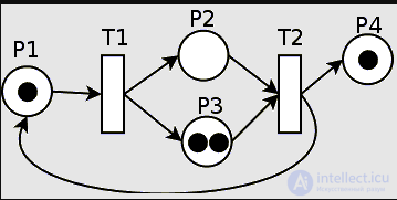
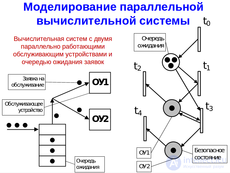
An example of a Petri net. White circles denote places, bars denote transitions, and black circles denote tokens.
A Petri net is a “place-transition” net N = (P, T, F, H, S), consisting of the following objects: P and T — disjoint sets into which the set of all nodes of the net is divided. Nodes from P are called places, or positions; nodes from T — transitions. The functions F and H specify, for each transition, the subset of places connected to it by arcs: F(t) — the set of input places of transition t, from which arcs enter t; H(t) — the set of output places, into which arcs leave t.
The function S labels the transitions, i.e. S(t) — the label of transition t (different transitions may be labelled identically).
Graphically, a Petri net (PN) is depicted as a bipartite graph, whose elements are positions and transitions, connected by directed arcs. A position is represented as a circle, and a transition — as a straight-line segment [19].
In analytical form, a Petri net can be represented as follows:

where B = {bj} — a finite nonempty set of positions; D — = {d,} — a finite nonempty set of transitions; / : B x D —> —» {0, 1} — the input function (direct incidence function), which for each transition specifies the set of its input positions; O: D x B ^ (0, 1} — the output function (inverse incidence function), which for each transition specifies the set of its output positions; M — the marking function of the net, M: B —> —> (0, 1, 2, ...}, which assigns to each position a nonnegative integer (equal to the number of tokens at that position).
To define the interpretation of the net, we need to introduce the notions of the state of the net and of the firing of a transition. The state, or marking, M — is a function which assigns to each place, in the simplest case, the value 1 or 0, indicating the presence or readiness at that place of objects for processing (the requests, data, resources, etc. required for processing), or their absence, respectively. Graphically, the presence of an object at a position is represented by a point called a marker. According to the classical definition of a PN, any position may hold an unbounded number of markers (any positive integer), i.e. the “capacity” of a position is unbounded. Therefore, to represent a bounded resource in classical PNs, special methods must be applied.
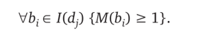
Given the notation introduced, the necessary condition for the firing of transition d, (for all input positions the number of markers located in them must be no less than 1) can be written as follows:
The firing of transition dt changes the marking of the net M(B) into the marking M'(B) according to the following rule:

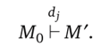
i.e. transition dj removes one marker from each of its input positions and adds one marker to each of its output positions. The change of marking is denoted as follows:
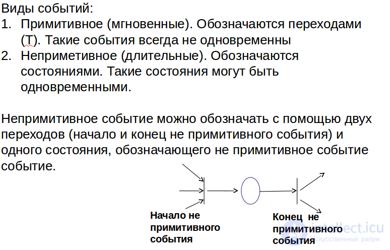
A simple representation of a system by a Petri net is based on two fundamental notions: events and conditions. Events — are actions that take place in the system. The occurrence of an event is governed by the state of the system. The state of the system can be described by a set of conditions. A condition — is a predicate, or a logical description of the state of the system. A condition can take the value either “false” or “true”.
Since events are actions, they can occur. In order for an event to occur, the corresponding conditions must be satisfied. These conditions are called the preconditions of the event. The occurrence of an event may cause the violation of preconditions and lead to the satisfaction of other conditions — postconditions.
In a PN, conditions are modelled by positions, and events — by transitions. Here the inputs of a transition are the preconditions of the corresponding event; the outputs — the postconditions. The occurrence of an event is equivalent to the firing of the corresponding transition. The satisfaction of a condition is represented by marker(s) at the position corresponding to that condition. The firing of a transition removes the enabling markers representing the satisfaction of the preconditions, and creates new markers representing the satisfaction of the postconditions.
A change of state occurs as a result of the firing of some transition, which becomes possible when all of its input places are ready; the label of a transition can be interpreted as the action performed when the transition fires.
Depending on the modelling objectives, the configuration components may vary.
Let us give the minimum information about PNs necessary to correctly understand the material presented and to construct PNs for the problems under consideration.
1. Elements of the same type in a PN cannot be connected to one another by arcs directly (Fig. 2.1, a).
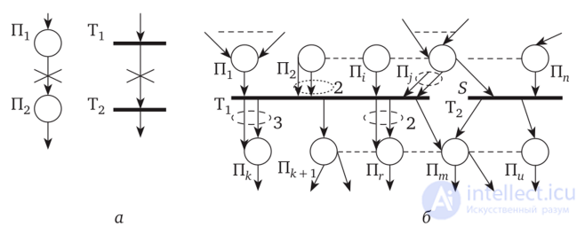
Fig. 2.1
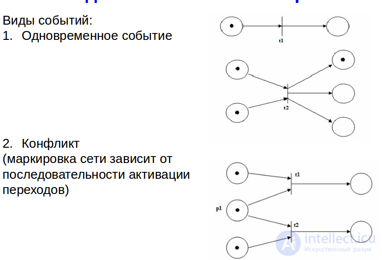
An event in a Petri net - is the firing of a transition in the net, in which tokens move from the input positions of that transition to the output positions. Events occur instantaneously, or at different times, upon the satisfaction of certain conditions.
Petri nets were developed for modelling systems with parallel interacting components. Petri nets were first proposed by Carl Adam Petri. In his doctoral dissertation "Communication with Automata" he formulated the basic concepts of the theory of communication among the asynchronous components of a computing system.
1 The concept of a Petri net. A Petri net is a bipartite directed graph containing vertices of two types — places (denoted by circles) and transitions (denoted by rectangles). Every arc leads either from a place-vertex to a transition-vertex, or vice versa. Arcs connecting two places or two transitions are forbidden. Places that have no incoming arcs are called input places. Places that have no outgoing arcs are called output places. Each place of a Petri net may contain zero or more tokens (also called markers). All tokens are considered identical and indistinguishable from one another. The distribution of tokens over the places of the net is called its marking. The operation of the net begins with an initial marking. Tokens can be moved from one place to another. The movement of tokens is carried out according to the following scheme.
• A transition is active (enabled) if each of its input places contains at least one token (more precisely — one token for each arc entering that transition).
• An active transition may fire; when it fires, the transition consumes one token from each of its input places and places one token on each of its output places (one token per outgoing arc).
• At each moment in time, one of all the active transitions is chosen nondeterministically to fire. If there are no active transitions, the operation of the net ends at that point. Let us assign to each transition of the Petri net some unique symbol (for example, number them). A sequence of symbols σ, in which the i-th symbol equals the symbol of the transition that fired at the i-th step
of the net's operation, is called the firing sequence of the Petri net. The firing sequence uniquely determines the sequence of markings µi , where µ0 is the initial marking. The fact that, after the firing of the t-th transition, the marking µ is transformed into the marking µ 0 , we will denote briefly as  . Figure 0.1 shows an example of the operation of a Petri net for the firing sequence σ = [t1, t3]. In each case, the active transitions are marked with an asterisk. Note that for the same net there is only one other possible firing sequence, σ = [t1, t2].
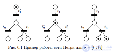
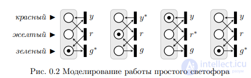
Figure 0.2 shows an example of modelling a simple traffic light with a Petri net, in which the colours switch in the following order (green, yellow, red), with the duration of each signal being the same (and equal to one clock cycle of the Petri net's operation). A distinguishing feature of this net is that its operation never terminates.
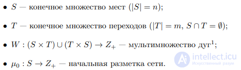
Formally, a Petri net is defined as a quadruple  , where
1By the symbol Z+ we shall denote the set of nonnegative integers
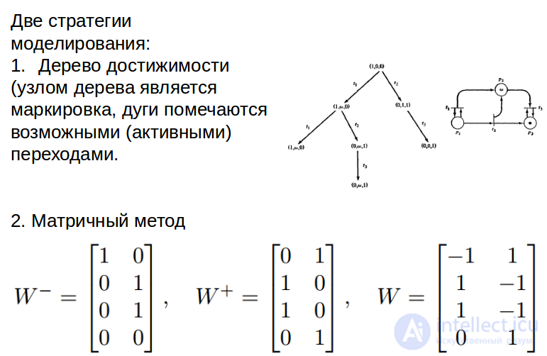
A Petri net can also be specified in a compact vector-matrix form. In this case, the structure of the Petri net (i.e. its graph) is described by two matrices W+ and W− of size n×m, defining the sets of arcs leading from places to transitions (matrix W−) and back (W+):  = the number of arcs leading from the i-th place to the k-th transition;
  = the number of arcs leading into the i-th place from the k-th transition.
From the matrices W+ and W−, one more matrix is formed,  , which is usually used to compute the new state (marking)
of the net after applying a given firing sequence to it.
The initial marking of the net is given by an integer vector µ0 of length n.
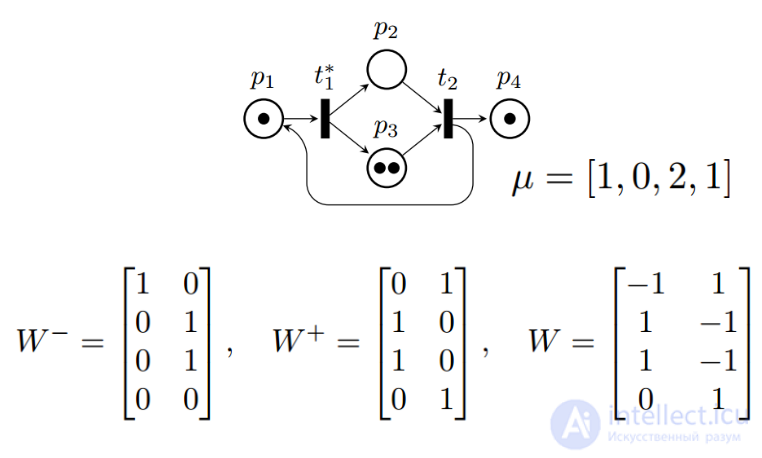
For example, for the net shown in Figure 0.3, the matrices W+, W− and W
are equal to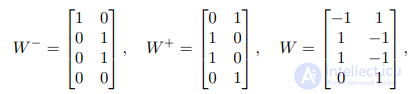
,
and its marking (on the left-hand side of the figure) is given by the vector µ = [1, 0, 2, 1]
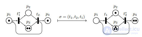
Fig. 0.3 Example of applying the sequence σ to a Petri net
It is easy to verify that, for the marking µ, the transition is active if the condition

holds. In the last formula, the symbol  denotes the k-th column of the matrix W−, and the comparison of two vectors is performed element-wise (i.e. it is taken that
a ≤ b if each element of a is less than or equal to the corresponding element of b:  for all possible i).
For the Petri net shown on the left-hand side of Figure 0.3, it is easy to verify that the following inequalities hold
This means that the first transition is active in this case, while the second is not.
Suppose that for some Petri net a valid firing sequence σ is given. Denote by v(σ) the vector whose k-th element is equal to
the number of occurrences of the symbol tk in σ. For example, for the net with two transitions (Figure 0.3) and the sequence σ = (t1, t2, t1), the vector v = [2, 1]. Then it is easy to verify that applying the sequence σ to the initial marking µ leads to the marking µ0, whose vector representation is computed by the following formula:

For example, applying the sequence σ = (t1, t2, t1) to the net shown on the left-hand side of Figure 0.3 will result in a marking that can be
computed by formula (1) as follows:
.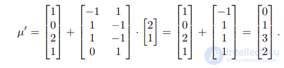
It can be seen that the result of this vector-matrix computation fully
corresponds to the marking of the net on the right-hand side of Figure 0.3.
At present, Petri nets are used mainly for modelling. In many fields of research, a phenomenon is studied not directly, but indirectly, through a model. A model is a representation, usually in mathematical terms, of what is considered most characteristic of the object or system under study. By manipulating a model of a system, one can obtain new knowledge about it while avoiding the danger, expense, or inconvenience of analysing the real system itself. Models usually have a mathematical basis.
The development of Petri net theory has proceeded along two lines. The formal theory of Petri nets is concerned with developing the basic tools, methods, and concepts necessary for applying Petri nets. The applied theory of Petri nets is concerned mainly with the application of Petri nets to the modelling of systems, their analysis, and the resulting deep insight into the systems being modelled.
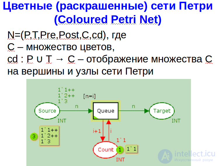
Modelling with Petri nets is carried out at the event level. It is determined what actions take place in the system, what states preceded those actions, and what states the system will assume after the action is performed. The execution of the event-based model in a Petri net describes the behaviour of the system. Analysis of the execution results can indicate which states the system was or was not in, and which states are in principle unreachable. However, such analysis does not provide numerical characteristics that determine the state of the system. The development of Petri net theory has led to the emergence of so-called "coloured" Petri nets. The notion of colour in them is closely related to the notions of variables, data types, conditions, and other constructs closer to programming languages. Despite certain similarities between coloured Petri nets and programs, they have not yet been used as a programming language.
Despite the advantages of Petri nets described above, the inconveniences of using Petri nets as a programming language lie in the process of their execution in a computing system. Petri nets have no strict notion of a process that could be executed on a specified processor. Nor is there a unique sequence of execution for a Petri net, since the underlying theory provides us with a language for describing parallel processes.
Petri nets possess the best capabilities for describing parallel systems. They are no less powerful than MPI, PVM, SDL, UML, and others, but in order to execute them on processors, it is necessary to turn the parallel description into a distributed one.
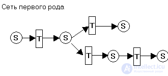
A first-kind Petri net - is a coloured Petri net described in a prescription language.
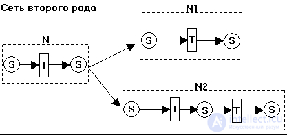
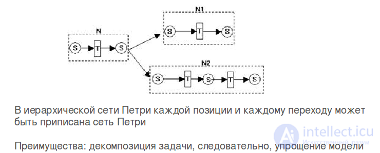
A second-kind Petri net - is a net represented as a hierarchical composition of objects.
The operation of a Petri net can be clearly represented by the reachability graph of markings. The state of the net is uniquely determined by its marking - the distribution of tokens over the positions. The vertices of the graph are the admissible markings of the Petri net, and the arcs are labelled with the symbol of the firing transition. An arc is constructed for each enabled transition. Construction stops when we obtain markings in which no transition is enabled, or markings already contained in the graph.
Note that the reachability graph of markings - represents an automaton.
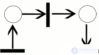
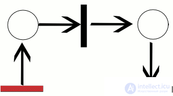
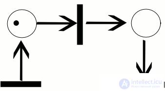
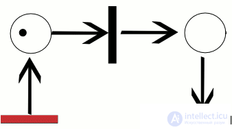
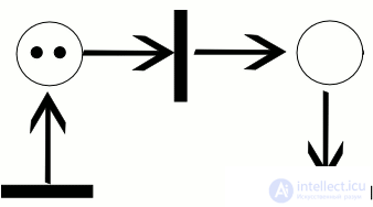
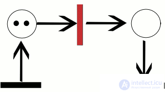
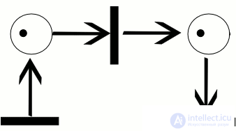
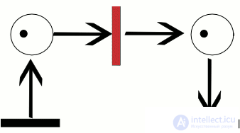
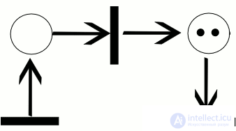
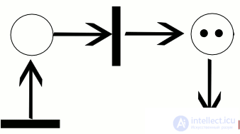
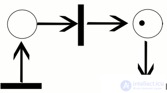
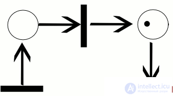
An example of a trajectory in a Petri net
Some kinds of Petri nets:
A timed Petri net - is a net in which transitions have a weight that determines the duration of firing (the delay).
A stochastic Petri net - is a net in which the delays are random variables.
A functional Petri net - is a net in which the delays are defined as functions of certain arguments, for example, the number of tokens in some positions, or the state of certain transitions.
A coloured Petri net - is a net in which tokens can be of various types, denoted by colours; the type of a token can be used as an argument in functional nets.
An inhibitor Petri net - is a net in which inhibitor, i.e. suppressing, arcs are possible, which forbid the firing of a transition if the input position connected to the transition by an inhibitor arc holds a token.
A hierarchical Petri net - is a net containing non-instantaneous transitions, into which other, possibly also hierarchical, nets are nested. The firing of such a transition characterises the completion of the full life cycle of the nested net.
WF Petri nets - a subclass of Petri nets, also called workflow nets. The formalism of WF-nets was introduced by Wil van der Aalst for modelling workflows in workflow systems.
A Petri net PN = (P,T,F) is called a workflow net (WF-net) if the following conditions hold:
WF-nets are used to check workflow graphs for structural conflicts such as "deadlocks" and "lack of synchronization". There are no structural conflicts if the WF-net is sound.
The property of soundness, of proper completion, - corresponds to the following requirements:
The soundness property corresponds to two well-known properties of Petri nets - liveness and boundedness.
Unlike Petri nets, in E-nets :
In connection with this, any transition can be described by a triple of parameters 
Here S — is the type of the transition, t(d,) — is the delay function, reflecting the duration of the transition's firing, p(<2;0 — is the function transforming the attributes of the tokens.
Another important difference between E-nets and Petri nets is that tokens are interpreted as transactions moving through the net, while transition-vertices are treated as devices performing some kind of processing of the transactions. A consequence of this approach is the requirement that no position-vertex may contain more than one token (i.e. any E-net is inherently safe).
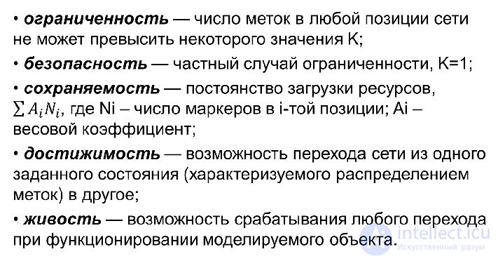
The main properties of a Petri net are:
The study of the properties listed above is based on reachability analysis. Methods for analysing the properties of Petri nets are based on the use of reachability (covering) graphs of markings, solving the state equation of the net, and computing linear invariants of positions and transitions. Auxiliary methods of reduction, which allow the size of a Petri net to be reduced while preserving its properties, and of decomposition, which split the original net into subnets, are also used.
In 1974, Tilak Agerwala showed that an inhibitor Petri net is a universal algorithmic system. In the monograph of V. E. Kotov, a sketch of the proof is given, indicating the rules for encoding, by an inhibitor net, the program of Minsky's counter automaton. J. Peterson gives examples of other extended classes of Petri nets that are universal algorithmic systems: synchronous and prioritised ones. A universal Petri net constructed explicitly numbered several thousand vertices and has recently been reduced to 56 vertices.
Infinite Petri nets were introduced for the verification of computational lattices and make it possible to determine the properties of Petri nets for regular structures (linear, tree-like, square, triangular, hexagonal, and hypercube) of arbitrary size, obtained by composing typical fragments.
The theory of Petri nets is a well-known and popular formalism intended for working with parallel and asynchronous systems. Founded in the early 1960s by the German mathematician C. A. Petri, it now contains a large number of models, methods, and analysis tools, which have an extensive range of applications in practically all branches of computer technology and even beyond it.
1. The root of the tree is a node labelled with the initial marking. Construction then proceeds.
2. If the value m(x)i = w. Then for the generated vertex z: m(z)i = w.
3. On the path from the root vertex to vertex x there exists a vertex y with a smaller marking m(y) < m(x), m(y)i < m(x)i. In this case the infinity symbol is generated: m(x)i = w, m(z)i = w. In the example considered on the next slide, such a vertex is, for instance, the vertex with the marking (1, 2, 0) -> (1, w, 0).
4. If an enabled marking exists, then this marking is entered into the generated vertex z in accordance with the rules of transition firing.
The algorithm terminates its work once all vertices are internal, terminal, or duplicate.
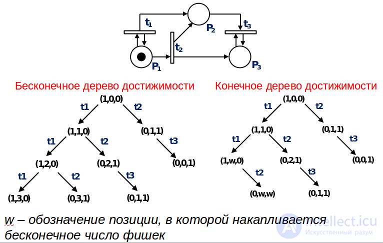
Types of vertices of the reachability tree:
The change in the marking of a Petri net is described by the formula:
µ ‘=µ +W*e
Where v – the transition vector
µ ‘ – the new marking

Places – data storage location;
Tokens – data being transmitted;
Transitions – data processing.
Places – data processing;
Tokens – data being transmitted;
Transitions – data storage location.
As Professor Carl Hewitt of the Massachusetts Institute of Technology, USA, notes, Petri nets have the following drawbacks:
they model the control flow, but not the data flow itself;
the difficulty of describing simultaneous actions occurring during a computational process;
the physical interpretation of a transition in Petri nets is quite dubious.
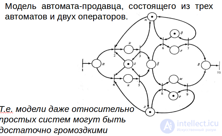
The cumbersomeness of Petri nets for modelling parallel processes

Comments