
Lecture
A reversible cellular automaton — a cellular automaton in which each state has a single predecessor. In other words, it is a regular lattice of cells, the state of each of which is taken from a finite set of states, together with a rule for simultaneously updating the states of the cells based on the states of their neighbours. The condition of reversibility consists in the fact that the previous state of any cell can be determined by knowing the updated states of all cells of the lattice. After reversing time one obtains another reversible cellular automaton, possibly — with much larger neighbourhoods, but likewise with a rule for determining the future state of a cell based on the current states of its neighbours.
Several methods are known for specifying reversible cellular automata, including block cellular automata, in which each block is updated independently of the others, and second-order cellular automata, in which the rule for updating cells is determined by the two previous states of the automaton. At the same time, if the automaton is specified by means of a rule table, the problem of checking its reversibility is decidable for a one-dimensional cellular automaton, but undecidable in the general case.
Reversible cellular automata provide a natural model for reversible computation — a technology that makes it possible to build computing devices with very low power consumption. Quantum cellular automata, which allow computation using the principles of quantum mechanics, are often assumed to be reversible. Moreover, many models from physics, such as the motion of molecules of an ideal gas or the Ising model of the arrangement of magnetic charges, are naturally reversible and are modelled by reversible cellular automata.
The properties inherent to reversible cellular automata can be used to study automata that are not reversible but that have an attractor — a subset of states to which random initial states converge. As Stephen Wolfram writes, “on approaching the attractor, any system, even an irreversible one, exhibits some properties close to reversibility” .
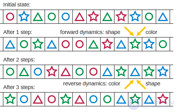
A one-dimensional reversible cellular automaton with 9 states. At each step, a cell takes the shape of its left neighbour and the colour — of its right neighbour.
The simplest cellular automata have a one-dimensional array of cells, each of which contains 0 or 1, with the neighbourhood of a cell consisting of the cell itself and one neighbour on each side; such cellular automata are called elementary . If the transition function never changes the state of a cell, always replaces it with the opposite one, replaces it with the state of a neighbour (always the same one — left or right), or applies a combination of the last two operations, then such an elementary cellular automaton is reversible. Despite its simplicity, the transition function that assigns to each cell the value of its neighbour plays an important role in symbolic dynamics, where it is known as the shift operator .
Elementary cellular automata are irreversible, apart from the trivial cases mentioned above, in which each cell is determined by the state of only one of its neighbours. However, close to reversible is rule 90, in which the future state of each cell is the sum modulo 2 (also known as exclusive “OR”, English XOR) of the current states of its two neighbours. Although rule 90 is irreversible, each of its configurations has exactly four predecessors, and rule 90 is also locally reversible, meaning that any sequence of consecutive states has at least one predecessor .
A slightly more complex example is obtained as follows: let the state of each cell be an ordered pair (l,r), and let the transition function take the left part of the new state from the neighbour on the left, and the right part — from the right. Here we assume that the left and right parts are taken from two different finite sets of possible values. An example is shown in the illustration at the beginning of the article: the left part of the state is the shape of the figure, and the right part is its colour. Such an automaton is reversible, since one can take the left part of the previous state from the cell on the right, and the right part — from the left.
Another example of a reversible one-dimensional cellular automaton produces multiplication by 2 or 5 in decimal notation. Each digit under such multiplication depends only on the two previous digits, and hence the neighbourhood determining the next value is finite, which is what is required for a cellular automaton. In general, multiplication or division of a number written in a positional system by a natural number n is defined by a cellular automaton if and only if all prime factors of n divide the base of the numeral system. Such an automaton is one-dimensional and reversible, since one can respectively divide or multiply by the same number. For instance, multiplication by 3 in decimal notation is not defined by a cellular automaton, since a carry may occur across an arbitrarily large number of digits: when multiplying 333334*3=1000002 a carry occurs across 5 digits .
The game “Life”, one of the best-known cellular automata, is not reversible: for example, many configurations die out. It also contains Gardens of Eden — configurations without predecessors. Instead, Tommaso Toffoli and Norman Margolus invented “Critters” — a reversible cellular automaton with dynamic behaviour largely similar to that of “Life” .
“Critters” is a block cellular automaton in which cells are divided into 2 × 2 blocks that are updated separately from the rest. After each step the partition into blocks changes: the blocks shift by one cell horizontally and vertically. The transition function of “Critters” changes the state of each cell to the opposite one if the number of live cells in the block is not equal to two, and rotates the whole block by 180° if that number equals three. Since the number of live cells changes into the number of dead cells, and the transition functions for each value of the cell count are reversible, such a cellular automaton is reversible on each block, and is therefore reversible overall .
If one starts with a small number of random cells inside a larger region of dead cells, many small patterns similar to the glider from the game “Life” spread out from the central region and interact in a complex manner. At the same time, “Critters” allows for complex spaceships and oscillators with an infinite number of different periods .
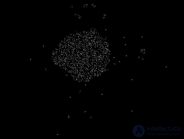
Gliders spread out from a central region set at random.
Several general methods are known for constructing reversible cellular automata.
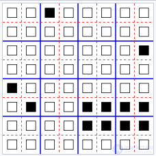
The Margolus neighbourhood for block cellular automata. The transformation rule acts in turn on 2 × 2 blocks bounded by blue lines, and 2 × 2 blocks bounded by dashed red lines.
A block cellular automaton — a cellular automaton whose cells are divided into equal blocks, and whose transition function is applied to each block separately. Such an automaton usually uses several block partitions in turn . A typical example of such a scheme is the Margolus neighbourhood, in which the cells of a square lattice are divided into 2 × 2 blocks by vertical and horizontal lines, and after each step the partition into blocks shifts by one cell horizontally and vertically; thus, all four cells of any block end up in different blocks at the next step . “Critters”, considered above, uses the Margolus neighbourhood.
For a block cellular automaton to be reversible, it is necessary and sufficient that the transition function be reversible on each block, which makes it possible to check the reversibility of a block cellular automaton by exhaustive search. Here the inverse cellular automaton is likewise a block automaton with the same structure of block partitions, but with the inverse transition function .
Any {\displaystyle d} -dimensional cellular automaton can be embedded in a
  -dimensional reversible one: here each state of the new automaton stores the entire history of the evolution of the old one. Using this embedding, Toffoli showed that many properties of irreversible cellular automata carry over to reversible ones, for example, they can be Turing-complete .
The increase in dimensionality in such a construction is not accidental: under certain weak restrictions (such as invariance of the embedding with respect to translations), it has been proved that any embedding of a cellular automaton with a “Garden of Eden”, that is, a configuration without predecessors, into a reversible cellular automaton must increase the dimensionality[10].
However, in the presence of quiescent states (English: quiescent states), that is, states that do not change provided that neighbouring states also do not change , it is possible to simulate a finite configuration of a cellular automaton in a block reversible cellular automaton of the same dimensionality[11]. Information that would otherwise be lost at the next step is instead stored in an infinite region of cells that are in the quiescent state. Here, the time required to simulate part of a configuration is proportional to its size. Nevertheless, such a construction makes it possible to prove the existence of a reversible one-dimensional cellular automaton that is Turing-complete[12].

Comments