
Lecture
Traffic flows are made up of individual trips undertaken by road users, or users of the transport network. In general, when speaking of trips, we include in this concept not only journeys by various
modes of transport, but also pedestrian trips. The main factors determining the number of trips made and their distribution across the transport
network of the city are:
The following types of traffic can be modelled and can interact with one another:
The construction of mathematical models requires a formal description of the factors listed above. The basis of such a description is the transport graph, whose nodes correspond to intersections and off-street transport stations, and whose arcs correspond to segments
of streets and off-street transport lines. The arcs also include arcs representing transfers from street-level to off-street transport. A separate component
of the transport graph is the route graph of public transport. The nodes of the route graph are stopping points, and the arcs are route segments between stopping points. The stop-nodes of the graph are connected to the ordinary nodes
by boarding arcs and alighting arcs.
To describe the distribution of trip-generating facilities, it is necessary to divide
the city into a certain number of conditional origin-destination zones (OD zones).
Each OD zone is included in the graph as a node connected to the ordinary nodes
of the graph by special connector arcs. The total volume of trips from one zone
to another OD zone (irrespective of the specific paths of travel) is called the inter-zonal correspondence.
The basis for modelling user behaviour is the mathematical
formulation of the criterion by which a user evaluates alternative paths and modes of travel. This criterion is customarily called the generalised cost of the path. An increase in the generalised cost reduces the attractiveness of the path. The generalised cost of a path is made up of the generalised costs of the arcs comprising it.
In addition, the cost of a path may include the cost of transitions from one arc to another, for example
the cost of a turn when travelling along the street-road network (SRN), or the cost of boarding when
transferring from a transfer arc to an arc corresponding to a trip.
An example of the evolution of a transport network and its network characteristics under the Erdős-Rényi model is shown in Figure 3.
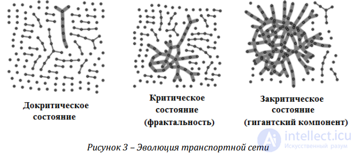
Figure 3 – Evolution of the transport network
The models used for analysing transport networks are highly diverse. At the same time, there is currently no exhaustive classification of modelling methods. Systematisations have been carried out according to different criteria depending on the problems being solved. For example, depending on the solution method – into analytical and simulation models [2, 6]; by data representation method – into dynamic models, which operate in real time, and static models, in which parameters are averaged over a certain time interval [16]. On the time scale, continuous and discrete models are distinguished [17]. By type of process representation, models are divided into stochastic models, which are based on a dependence on a random combination of parameters, and deterministic models, in which the next state of the traffic flow is uniquely determined on the basis of the previous one [15]. Based on the functional role of the models, three main classes can be conditionally distinguished [16]: forecasting models, simulation models, and optimisation models. This classification does not reflect the solution method, nor the assumptions underlying the model.
The most popular classification is by the level of detail of the traffic flow [22], which distinguishes macroscopic models, mesoscopic models, microscopic models, and submicroscopic models. However, this classification gives no indication of either the field of application or the modelling method.
In the view of the authors of this work, the following classification of traffic flow models is possible, based on two main criteria: the level of detail and the modelling method.
– Macroscopic:
– Mesoscopic:
– Microscopic:
This classification takes into account both the modelling methods and the degree of detail. Let us examine some of the models listed above in more detail.
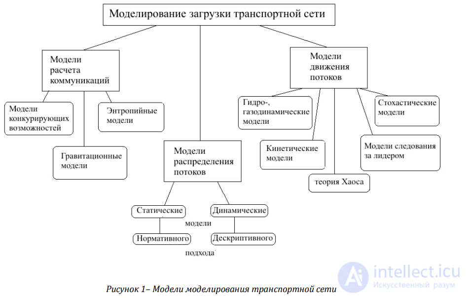
Figure 1 – Models for modelling the transport network
Analogue modelling describes the motion of vehicles as the flow of a specific fluid. During modelling, the averaged characteristics of the flow are studied, such as density, average speed and traffic volume, but individual vehicles are not considered. Macroscopic models may be continuous, described by partial differential equations, or discrete. Hydrodynamic models may or may not take inertia into account. Models that disregard inertia are often derived from the continuity equation and treat speed as a function of density. This makes it possible to describe the motion of a locally equilibrium flow [14]. Models based on the Navier – Stokes equations take the effect of inertia into account and describe drivers’ tendency to travel at their desired speed.
Let us consider common examples of methods that most accurately reflect the main characteristics of the macroscopic approach [3, 11]. The Lighthill – Whitham – Richards (LWR) model [19] belongs to the analogue models; it is based on the equations of hydrodynamics and on the fulfilment of the law of conservation of mass, where mass is taken to mean the number of vehicles. The LWR model does not work at very low or very high traffic densities and is inadequate near “bottlenecks” and signalised intersections. Nevertheless, the hydrodynamic approach became the basis for more advanced models. Thus, in 1971 Payne [18] proposed describing the dynamic relationship by means of a differential equation of convection type (the equation was derived from a car-following model). Payne’s model should be understood as a conservation law, but because speed does not depend on density, a right-hand side is introduced into the equation – the conservation of momentum. Phillips took into account the internal pressure of the flow, which makes drivers react in a manner similar to the actions of the leading vehicle [21]. The Greenshields model (1934) contains a linear relationship between density and speed. It was later modified by Richardson. In the Greenshields model, when determining capacity it is important to choose the free-flow speed correctly. Otherwise, too high a value leads to overestimated results, which is confirmed in [11]. The last two models share one feature: the lower the free-flow speed, the more closely the calculated data match the experimental data. The Greenberg and Al-Hozaini macromodels have a logarithmic relationship between traffic density and speed [17]. The Greenberg model has a serious drawback: as traffic density tends to zero, the speed value can become greater than the free-flow speed. The Al-Hozaini model works adequately when a high flow density is given and its speed is not less than 17 km/h. The Underwood, Drake and Zyryanov models have an exponential relationship between the density and speed of vehicular flow. These models share one common drawback: if the traffic density value is sufficiently large, the resulting flow rate will exceed the actual value. The models of D. Drew and L. Pipes have a power-law relationship between density and speed [17]. A feature of these models is that they can be fitted to experimental data by means of a proportionality coefficient.
As a result of applying macroscopic models, one usually determines the travel time, average speed, network load level, and traffic volume. Modelling at the macro level has certain advantages [12]: low computer requirements and high calculation speed. However, it also has drawbacks: the results obtained are static and not sufficiently accurate; the initial data needed for solving problems are difficult to determine.
Meso-modelling describes motor vehicles fairly precisely, but at the same time considers their interaction and behaviour in the same way as at the macro level [10, 16, 13]. The gravity model is considered one of the first models to reflect the interaction of a pair of zones that generate traffic flows (trips). It was based on the law of universal gravitation. Among its drawbacks is the fact that the total number of trips is linked to only one pair of zones. However, visits may depend on the position of the destination zone relative to other zones. This drawback is addressed in the models of the competing-destinations family. The use of the concept of entropy for solving transport problems was proposed by Wilson [4, 24]. This model is based on the second law of thermodynamics. A transport system resembles a physical system in that it contains a large number of uncontrolled elements. For this reason, it has been proposed to replace the problem of determining trips with the maximisation of entropy in the transport system [15].
In the equilibrium assignment model it is assumed that all road users choose their routes based on the minimum travel cost. As a result of the “trial and error” process, an equilibrium flow assignment is established in the system, possessing properties known as Wardrop’s conditions [23]. The essence of these properties is as follows: under an equilibrium assignment of vehicles, no road user changes their route, because the travel cost is already minimal.
The main advantage of the models listed above is their relative compactness. However, these models have a number of drawbacks: they cover only a limited set of parameters (speed, delays, queues) and take little account of the dynamics of traffic flow.
The basic traffic model defining the movement of vehicles was developed by Rainer Wiedemann in 1974 at the University of Karlsruhe. It is a car-following model that takes into account the physical and psychological aspects of drivers.
The model underlying pedestrian dynamics is the Social Force Model, developed by Dirk Helbing et al. in 1995.
“Microscopic modelling”, sometimes called microsimulation, means that every object of reality (a car, a train, a person) is modelled individually, i.e. by a corresponding entity in the model, thereby taking all relevant properties into account. The same applies to interactions between entities. The opposite of this would be “macroscopic modelling”, in which the description of reality shifts from individual entities to “averaged” variables such as flow and density. The corresponding product from the same manufacturer is so named. Wikipedia site:tftwiki.ru
These models describe the motion of each vehicle individually. Micromodels became popular after the advent of powerful computers, since they required a large volume of calculations. Such models are well suited to representing movement on roads with several lanes, because they can describe realistic rules for vehicle movement [5, 8, 15, 19]. The “car-following” model was one of the first; it was developed by A. Reuschel (1950) and L. Pipes (1953). The basic idea lies in the influence of the lead vehicle on the vehicles following it. The leader’s influence is expressed indirectly through the dependence of the optimal speed on the distance to the vehicle ahead. Over time the theory was developed further and modified; in particular, drivers’ reaction time began to be taken into account, movement on multi-lane roads was studied, and the stability of traffic flow was investigated. In 1959, engineers at the General Motors automotive corporation proposed their own microscopic model for describing a single traffic lane, with which the fundamental diagram can be obtained. The next step was Newell’s model [20], presented in 1961. The basic assumption is as follows: each driver has their own “safe” speed, which depends on the distance to the leader. In this model it is important to choose correctly the function relating speed to the spacing between vehicles. Drivers’ reaction time should be chosen with care: values that are too large produce collisions, while values that are too small can produce unrealistic accelerations. The last two models considered can be combined into one general “intelligent driver” micromodel. It was proposed by Treiber in 1999. Motion in the model is described as a combination of two strategies: acceleration and braking. Priority is given to one or the other depending on the distance to the vehicle ahead. The intelligent driver model takes into account the psychophysical parameters of people, which helps to model traffic flows more realistically by randomly selecting the parameters of drivers.
Car-following models do not correctly describe the dynamics of an individual vehicle, which allows us to classify them as mesoscopic models. There is also a paradox in these models – if there is no leader, the acceleration becomes equal to zero.
Cellular automata have proved to be a very convenient apparatus for implementing microscopic models. Such a model was proposed by J. von Neumann in the early 1950s. In cellular-automaton models, the road is divided into cells and time is treated as discrete. Each cell can be in some state, which is determined by a set of rules depending on the states of neighbouring cells. Random perturbations introduce an element of stochasticity. The advantage of this approach is its high efficiency in computer modelling. Its drawback, however, is the relatively low accuracy at microscopic scales, owing to the discrete nature of the cellular automaton.
As a result of running microscopic models, the following data are typically obtained: queue length, vehicle delay time, average speed, maximum or minimum speed, and vehicle travel time. The main advantage of microscopic models is the possibility of obtaining estimates with high accuracy. However, the high level of detail in micromodels entails the following drawbacks: a large amount of resources is required to collect the initial data; a large number of model runs are needed to obtain reliable results; parameter calibration is necessary; there is high sensitivity to errors in the initial data; and there are difficulties in obtaining analytical relationships [15].
It should be noted that many approaches can be applied to describe processes in transport networks. For example, queueing theory [3-5], Petri nets [6,7], fuzzy set theory [8,9], cellular automaton theory, and much more. Despite existing developments and specific solutions in the field of control, transport networks are, from the standpoint of mathematical modelling and control, very complex and poorly studied objects requiring further research. At present, there are many implementations of software packages for modelling traffic flows. D
As a rule, in all programs, traffic flow modelling takes place at the micro level. We will therefore begin our review with it. Let us consider the most common models.
The gravity model.
Historically, one of the first mathematical models proposed for estimating interzonal trips was the gravity model ]. Let us consider a system consisting of a certain set R of zones
of origin and destination, connected to one another by routes across the transport network. The input data for calculating the trip matrix are:
Oi — the volume of departures from zone i ∈ R,
Dj — the volume of arrivals in zone j ∈ R.
Depending on the type of trip, volumes may be measured in vehicles,
passengers, or other convenient units. The following balance condition for total
arrivals and departures is assumed to hold
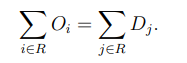
If the initial data do not satisfy this condition, the data must be adjusted by multiplying by a constant coefficient.
The gravity model is based on the following simple premise: the trips from zone i to zone j are proportional to the total volume of departures from centre i, the total volume of arrivals at centre j, and some function C(tij ), which depends on
the transport distance tij between centres i and j. Intuitively,
the transport distance reflects the degree of proximity between zones, taking into account the speed and
convenience of travel provided by the transport network. The method for determining
this quantity may differ between different variants of the model.
When calculating a homogeneous trip matrix, i.e. one made up of trips of a single type and users of a single class, the numerical expression of the transport distance is the generalised cost (in the particular case
the travel time) of the optimal (shortest) route connecting two zones. If
mixed trips are being estimated, for example including trips both by
public transport and by car, it is necessary to calculate the optimal
cost of travel by different modes of transport  , where k are the types of trip. As
the transport distance one can then take the weighted average of these costs
taking into account the split coefficients of trips by travel type:

) - split coefficients of trips into travel types as functions of the set of optimal travel times for the different types;
these coefficients satisfy the condition 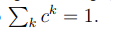
Let us denote by Fij the trips from zone i to zone j. Then the gravity model can be formulated as

where the coefficients are determined from the conditions
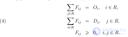
The function C(t) is called the deterrence function. It is the main factor determining the distribution of trips by distance, which is why the term settlement curve is also used. In some publications this function is interpreted as the “a priori probability of a trip originating” depending
on distance, although in the general case it need not satisfy any normalisation conditions. This function is chosen during calibration of the model
by comparing the output modelled distribution of distances with survey data. A large number of studies have been carried out on the calibration of this
function for different cities. In practical calculations,
the following approximation is often used:

The kinematic model is based on the elementary kinematic equation, in order to determine the maximum degree of acceleration or deceleration that a vehicle must exhibit to avoid a collision with another vehicle moving ahead of it. In each time-step, the new value an+1must be high enough to avoid a collision within the chosen time interval, which is called the time to collision – tc. In addition, it is necessary to continually change the distance Dx, in order to reach a certain optimal value for the next interval dx. Speed is adjusted so as to remain within the range [0 … Vmax].
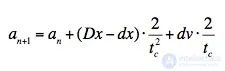
Since the model relies on only 2 parameters, the effort required to calibrate it is fairly low. But the modelling will obviously not achieve a high level of plausibility either. Because of its limitations, the kinematic model carries very little weight in modern traffic-flow modelling and is not recommended for use in determining the width of a roadway. It is included in the curricula of many European universities purely for educational purposes.
The entropy model.
The use of the concept of entropy for solving transport problems was proposed by Wilson, and this approach was subsequently developed in many works. The entropy model proceeds from a probabilistic description of the behaviour of network users. Network users are randomly distributed
over some set of possible states. When calculating trips, a user’s state can be taken to be their membership of a trip from i to j.
The independent and random choice of states by all users leads to
one or another macroscopic state of the system. According to the basic concept
of the entropy model, the state of the system that is realised in reality is the state with the greatest statistical weight. The use of the statistical weight
of states instead of the probability distribution of particular states is explained
by the fact that in entropy models a finite, normalised probability distribution may not exist. The statistical weights of states reflect the relative probabilities of different states being realised in the system. Bearing this
reservation in mind, states with the greatest statistical weight are also often called
the most probable states.
Mathematically, the state with the greatest statistical weight is defined as the
state that maximises a certain function in the state space,
called the entropy of the system. As applied to the problem of determining trips in a transport network, entropy is defined by the following expression:

Here fij — are the occupation numbers of the states, i.e. the numbers of system elements found in states (i, j). The quantities νij have the meaning of “a priori most probable” values of fij . The actual most probable values Fij are determined
from the solution of the entropy-maximisation problem under a certain system of constraints
on fij . In the absence of constraints, the solution of the maximisation problem leads to the a priori values Fij = νij . The constraints imposed on the distributions can
be of very different natures. As a rule, these constraints reflect the available information about the macroscopic characteristics of the state of the system. In the system
of constraints used in entropy models of transport networks, one can distinguish a group of standard linear constraints expressing the balance of arrivals
and departures. This group of constraints is also called the transport constraints. Taking the above into account, the entropy model for calculating trips can
be written in the form
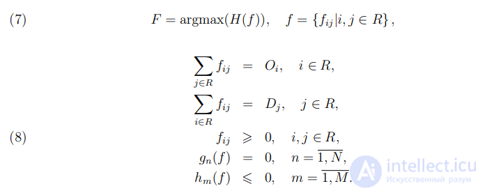
Here the transport constraints are explicitly singled out, and N
additional equality constraints and M inequality constraints are included in general form. The optimisation problem (7)-(8) is a standard mathematical programming problem
with a convex objective function. The system of constraints in this problem is, as a rule,
linear. The solution of the problem can, in general, be obtained by the method of Lagrange multipliers. In the particular case where only the transport constraints are present,
an analytical expression for the solution of problem (7)-(8) can be obtained. This expression coincides with the expression given by the gravity model if the a priori
probabilities are set in accordance with the deterrence function: νij = C(tij ). Another
way of establishing the connection between the entropy model and the gravity model was proposed
in [112]. Suppose that trips between the zones of arrival and departure
i and j are associated with a certain amount of “generalised cost”. Let the total
cost of travel be known for each departure zone:

These equalities can be used as constraints in the entropy-maximisation problem. They are called cost constraints. Let us consider an entropy problem in which the a priori probabilities of particular trip values are equal: νij = const, and the constraints include both balance and
cost constraints. The solution of the problem will also coincide in form with the expression given by the gravity model if we take tij = cij and use a deterrence function
of the form

The coefficient λ in this expression is the Lagrange multiplier of the optimisation problem;
its value is determined in the course of solving the problem itself. According to this reasoning, the entropy model can serve as a statistical justification for the gravity model, and moreover provides a basis for choosing the deterrence function.
Within the framework of the entropy-maximisation problem, it is also possible to calculate trips with simultaneous splitting by mode of travel. According to the general approach, we shall assume that the random state of a transport-network user consists in belonging to a trip from i to j and choosing a mode of travel k. The state of the system is then defined by a three-index set
 . The expressions for the entropy function and the corresponding maximisation problem are entirely analogous to (6)-(8). In this case, additional constraints on the total volume of travel for the different modes must be included among the constraints.
The probabilistic BANDO model. In 1995, Bando and his colleagues presented the so-called “optimal velocity model” (Optimal Velocity Model). It is a density-speed model that belongs to the group of deterministic leading models and links the target speed of vehicles to the macroscopic density of the traffic flow. Bando derived the optimal speed such that each vehicle would try to follow the relationship below:
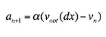
where:
an+1– acceleration for the next time interval;
α – the sensitivity factor (the value inverse to the reaction time of the
driver);
vopt – the optimal velocity function;
dx – the change in distance to the preceding vehicle;
vn – the current speed of the vehicle.
Bando’s team proposed an optimal velocity function that increases monotonically, with an upper bound of vmax.

Over time, the model was modified with several further optimal velocity functions. For example, by using different acceleration functions, or by differentiating between the free-flow speed of the vehicle (unsaturated traffic flow) and the speed-at-capacity (saturated traffic flow), using a 4-parameter equation (Van Aerde, 1995).
The probabilistic GAZIS model. The so-called car-following theory (“chasing the leader”), based on the research of Gazis, Herman and Rothery (1961), attempts to follow the behaviour of a vehicle by determining the distance, taking into account the driver’s reaction time to particular stimuli (for example, different speeds of the vehicle ahead), according to the formula:
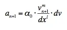 where:
an+1 – acceleration after the reaction time tp;
α0 – the sensitivity factor;
m, l – calibration parameters (coefficients);
dx – the speed difference relative to the preceding vehicle.
For German motorways, the values of the parameters m and l were established in the studies of Hoefs (1972) for various scenarios (a vehicle ahead moving away or approaching, with or without brake lights). However, owing to the steady increase in the number of vehicles on European motorways, during the development of the BABSIM modelling package the reference parameters were recalibrated, which led to new sets of parameters and more realistic modelling results.
Sparmann’s probabilistic lane-change model. Building on Wiedemann’s work, Sparmann developed a lane-change algorithm for a two-lane highway (Sparmann, 1978). Taking into account all six potential interaction partners (i.e. each vehicle ahead and behind in the current lane, as well as in the two adjacent lanes), a vehicle could change lane using Wiedemann’s parameters. As soon as the need for a lane change arises, a check is carried out – whether such a manoeuvre would endanger it or its so-called “interaction partner”. If the safety of all vehicles is ensured, the lane-change process begins and the vehicle ends up in the adjacent lane. One drawback of Sparmann’s model – the lack of a more anticipatory strategic approach. Only neighbouring vehicles are considered, ignoring the need of other vehicles to change lane.
THEIS probabilistic lane-change model. Theis (1997) added a strategic component to Sparmann’s model: if a vehicle tries to move into a particular lane, it must first “ask” for help from neighbouring vehicles. Conversely, the vehicle involved in the interaction must decide whether to accelerate or decelerate in order to create a gap for the lane-changing vehicle, or to change lane itself in order to make room for it.
The WIEDEMANN model as part of the PTV Vision VISSIM software package. Simulation modelling. The VISSIM simulation system consists of two separate programs that interact with each other via an interface, through which measurement data from detectors and data on the states of control systems are exchanged. The result of the simulation is an animation of traffic movement in the form of real-time graphics and the subsequent output of various traffic-engineering parameters, such as, for example, the distribution of travel time and waiting time broken down by user groups.
The traffic flow model incorporates a car-following model, intended to represent movement in a queue behind the vehicle ahead within a single traffic lane, and a lane-changing model. Traffic-dependent control logic is modelled using external programs that control traffic signal installations. The logical control program polls detector parameters at a cycle ranging from 1 second to 1/10 second (depending on the configuration and type of the traffic light installations). From the values obtained and the time intervals, the program determines the state of all control systems for the next simulation step and introduces them into the traffic flow simulation.
What is essential for the accuracy of the simulation system is the quality of the traffic-flow model, i.e. the method by which the movement of vehicles through the network is calculated. Unlike simpler models, which take constant speeds and unchanging car-following behaviour as a basis, PTV Vision® VISSIM uses Wiedemann's psycho-physiological perception model (1974, 1999). The basic idea of the model is that the driver of a vehicle travelling at a higher speed begins to brake on reaching their individual perception threshold with respect to the distance from the vehicle ahead, when the gap to the vehicle ahead begins to be perceived as too small. Since the driver cannot accurately judge the speed of the vehicle ahead, their speed will fall below the speed of the vehicle ahead until they begin to accelerate slightly again after reaching their perception threshold, when they begin to perceive the gap that has arisen between them and the vehicle ahead as too large. This leads to constant slight acceleration and deceleration. Distribution functions for speed and distance are used to simulate the differing behaviour of drivers.
Simulation models of this type belong to the car- following family:
Models of the car-following family focus on the characteristics of the individual vehicle. The Wiedemann model of the PSM class has the advantage in terms of the number of factors taken into account in microscopic-level modelling of traffic. The Wiedemann model incorporates the characteristics of the driver and of the vehicle itself, and represents a golden mean between cellular automata and the other classes of models within the car-following family.
Following numerous empirical studies carried out by the Karlsruhe Institute of Technology, this car-following model became the benchmark. More recent measurements show that the driving style and the technical capabilities of vehicles, which have changed in recent years, are correctly reflected in this model.
On multi-lane carriageways, the driver in the VISSIM model takes into account not only the vehicle ahead but also vehicles in both adjacent lanes. The driver's attention is additionally drawn in particular to a traffic light 100 m before reaching the stop line.
In VISSIM so-called driver–vehicle units move through the network. Each driver, with their own individual behavioural parameters, is associated with a specific vehicle. In this case, the driving style matches the technical capabilities of the vehicle.
At this stage, simulation modelling appears to be a powerful tool for evaluating and analysing the movement of vehicular and pedestrian flows. In addition, a program at the level of PTV Vision® VISSIM allows the designer's work to be considerably simplified and creates a reliable platform for designing both road-transport facilities and any other urban-planning objects.
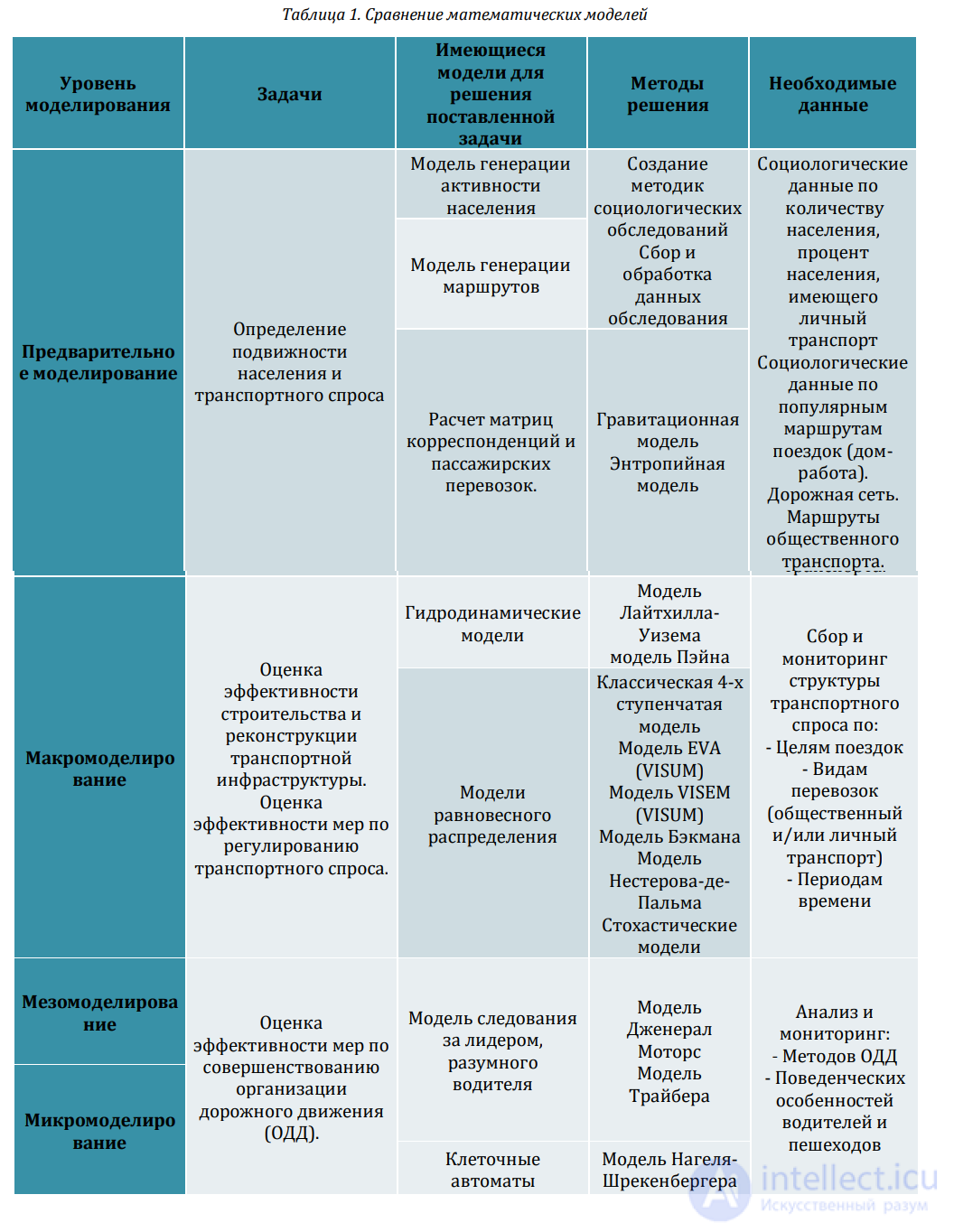
Table 1. Comparison of mathematical models

Comments